![[MAP Logo]](../../maplogo1.gif)
Billy Chan, Ph.D., P.Eng.,
MIL Systems,
1150 Morrison Drive,
Ottawa, Ontario,
Canada, K2H 8S9.
bchan@MILSystems.com
Program added: June 1999
NNWork is a MS-DOS based graphics program which uses a backpropagation neural network paradigm for analyzing empirical data, and enabling predictions to be carried out. A number of data files are provided which can be used for predicting cetain weld parameters: the heat affected zone hardness, the 800 to 500 °C cooling time, t8/5, and the weld dimensions.
Complete program. Also included are a number of data files which can be read by the program.
| Language: | Source code not available. |
| Product form: | Executable file for IBM-PC, PC/AT or compatible with at least 1M RAM, MS-DOS version 3.3 or later, a high resolution monitor (at least 640x348 active pixels) and a floppy disc drive with 300k free disc space. An Intel 486 processor with hard disc is highly recommended. Optional equipment: mouse (Microsoft or Logitech compatible) and dot matrix or HP II LaserJet (PCL compatible) printer. |
Backpropagation network (BPN) is an artificial neural network modelling paradigm which is well known for its prediction and data-mapping characteristics. i.e. it is capable of acquiring a knowledge about a relationship between input-output data sets in training and subsequently predicting an outcome for any given input data set within the knowledge domain of interest. An introduction to BPN is given in Appendix 1 of the manual: The outputs are linked to the inputs via an internal network (neural network) of points (nodes) which are arranged into a series of layers (hidden layers). Experimentally determined values of the inputs and outputs are used in the training process to determine suitable values for the strength of the links between each node of the network. Once these have been determined, they can be used to predict an outcome for any given set of inputs (within the range of values used for training).
The program is split into the three modules:
A series of weights files are provided which can be used to make predictions of HAZ (heat affected zone) hardness, the 800 to 500 °C cooling time, t8/5, and the weld dimensions.
The cooling time is obtained using the plate temperature, the plate thickness and the energy input rate per unit length as inputs to the network. The energy input rate, H, is calculated from the welding current, voltage, speed and efficiency using the equation H=efficiency.voltage.current/speed. The following weights files are available:
| T-20-53.WT2 | Network: 2 hidden layers with 5 and 3 nodes. |
| T-20-5.WT1 | Network: 1 hidden layer with 4 nodes. |
| T-20D.WT2 | Network: 2 hidden layers with 4 and 3 nodes. |
Twenty data-sets were used to produce the weights files. They were obtained from various sources and are given in Appendix III of reference 1. The maximum and minimum values of the inputs and outputs for the training data-sets used are:
| Plate thickness: | 12.7 - 63 mm. | Heat input: | 0.49 - 9.69 kJ/mm. | |||
| Plate temperature: | 15 - 155 °C. | Output t8/5: | 3.1 - 96.8 s. |
The most accurate results can be obtained using T-20-53.WT2, which made predictions with a mean error of 14%. These weights files can also be used for making predictions for other welding processes provided an appropiate value for the welding efficiency is given. Good agreement with experimental data over the valid input range was obtained for gas metal arc welds (GMAW) when a value of 70% (rather than 80%) was used for the efficiency.
The HAZ hardness of welds can be obtained given the composition of the weld material and the 800 to 500 °C cooling time. The material composition is specified in terms of the carbon concentration and two values for the carbon equivalent from references [2] and [3] respectively:
where C, Si, Mn, Cu, Cr, Ni, Mo, B and V refer to their corresponding concentrations in wt%. The data used for training the network was taken from the paper by Yurioka [4]. The following weights files are available:
| H50-4A2.WT1 | Network: 1 hidden layer with 4 nodes; 50 data-sets used for training. |
| Inputs: | carbon concentration, CE, Pcm, t8/5 |
| H50-53B.WT2 | Network: 2 hidden layers with 5 and 3 nodes; 40 data-sets used for training. |
| Inputs: | carbon concentration, CE, Pcm, t8/5 |
| H41-4C.WT1 | Network: 1 hidden layer with 4 nodes; 41 data-sets used for training. |
| Inputs: | carbon concentration, CE, Pcm, t8/5 |
| PCM50-4A.WT1 | Network: 1 hidden layer with 4 nodes; 50 data-sets used for training. |
| Inputs: | carbon concentration, Pcm, t8/5 |
| CE50-4C.WT1 | Network: 1 hidden layer with 4 nodes; 50 data-sets used for training. |
| Inputs: | carbon concentration, CE, t8/5 |
| CE41-4D.WT1 | Network: 1 hidden layer with 4 nodes; 41 data-sets used for training. |
| Inputs: | carbon concentration, CE, t8/5 |
| C41SI-4C.WT1 | Network: 1 hidden layer with 4 nodes; 41 data-sets used for training. |
| Inputs: | carbon and silicon concentrations, CE, t8/5 |
| SI43-4-1.WT1 | Network: 1 hidden layer with 4 nodes; 43 data-sets used for training. |
| Inputs: | carbon and silicon concentrations, CE, t8/5 |
| SIB-4A.WT1 | Network: 1 hidden layer with 4 nodes; 41 data-sets used for training. |
| Inputs: | carbon, silicon and boron concentrations, CE, t8/5 |
The maximum and minimum values of the inputs and outputs for the training data-sets used are:
| Carbon concentration: | 0.045 - 0.245 wt%. | Pcm: | 0.181 - 0.349 wt%. | |||
| Silicon concentration: | 0.164 - 0.436 wt%. | CE: | 0.381 - 0.549 wt%. | |||
| Boron concentration: | 0 - 0.0018 wt%. | t8/5: | 6.16 - 56.84 s. | |||
| Hardness (HVN): | 215.8 - 469.2 wt%. |
The most accurate results can be obtained using H50-4A2.WT1, which made predictions with a mean error of 3%. The weights files which were produced using only one value for the carbon equivalent as an input, made less accurate predictions but nevertheless had a mean error of less than 4%. SIB-4A.WT1, which included the boron concentration explicitly, produced results of comparable accuracy to the other weights files. However, it is likely to be unreliable due to an uneven distribution of boron content in the training data-sets.
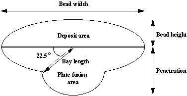
The weld bead geometry is defined in terms of the bead width, bead height, penetration, the (upper bead) deposit area (A1), the (lower bead) plate fusion area (A2) and the 22.5° lower bead bay length. (The bay angle was measured and found to have a mean value of 22.4° with a standard deviation of 8.2°.)
The data sets, obtained from bead-on-plate gas-metal-arc welds with either C-25 (25% CO2 and 75% Ar) or M-2 (2% O2 and 98% Ar) shielding gas, are given in Appendix VI of reference 1. The weld bead geometry was measured as a function of welding current, voltage, wire speed travel and plate thickness. Other welding parameters remained constant: electrode extension = 19.05mm; electrode diameter = 0.89mm, polarity = negative; efficiency = 70%. The following weights files are available:
| C25-BW.WT1 | Output: bead width; mean error = 5%. |
| C25-BH.WT1 | Output: bead height; mean error = 7%. |
| C25-PENE.WT2 | Output: penetration; mean error = 12%. |
| C25-225.WT1 | Output: low bead bay length; mean error = 7%. |
| C25-A1.WT1 | Output: deposit area (upper bead); mean error = 12%. |
| C25-A2.WT1 | Output: plate fusion area (lower bead); mean error = 12%. |
| Welding current: | 169 - 311 Amps. | Welding speed: | 3.8 - 10.6 mm/s. | |||
| Welding voltage: | 21 - 41 Volts. | Plate thickness: | 6.9 - 15.3 mm. |
| M2-BW.WT1 | Output: bead width; mean error = 7%. |
| M2-BH.WT1 | Output: bead height; mean error = 8%. |
| M2-PENE.WT2 | Output: penetration; mean error = 17%. |
| M2-225.WT1 | Output: low bead bay length; mean error = 15%. |
| M2-A1.WT1 | Output: deposit area (upper bead); mean error = 12%. |
| M2-A2.WT1 | Output: plate fusion area (lower bead); mean error = 18%. |
| Welding current: | 169 - 311 Amps. | Welding speed: | 4.5 - 9.0 mm/s. | |||
| Welding voltage: | 25 - 36 Volts. | Plate thickness: | 6.9 - 15.3 mm. |
| BW.WT1 | Output: bead width. |
| BH.WT1 | Output: bead height. |
| PENE.WT2 | Output: penetration. |
| 225.WT2 | Output: low bead bay length. |
| A1.WT1 | Output: deposit area (upper bead). |
| A2.WT2 | Output: plate fusion area (lower bead). |
| C25INV.WT2 | Inputs: bead width, bead height, penetration, lower bead bay length, plate thickness. |
| INV-WPA2.WT2 | Inputs: bead width, penetration, plate fusion area, plate thickness. |
| INV-WPAA.WT2 | Inputs: bead width, penetration, deposit area, plate fusion area, plate thickness. |
| INV-WAA.WT1 | Inputs: bead width, deposit area, plate fusion area, plate thickness. |
| Bead width: | 8.4 - 16.2 mm. | Lower bead bay length: | 2.1 - 4.7 mm. | |||
| Bead height: | 2.2 - 4.1 mm. | Deposit area: | 8.9 - 23 mm2. | |||
| Penetration: | 1.8 - 5.9 mm. | Plate fusion area: | 4.2 - 16.6 mm2. |
Files for Downloading
Installing and Running NNWork
Place nnwork.exe, nnwork.ovr and the *.hlp files into the same directory on either the hard disc or floppy disc.
To start the program either type nnwork at an MSDOS prompt
or (in windows) double click on the file nnwork.exe. The function keys can be used to enter the different modules (<F* NORM>,<F* TRAIN> and <F* USE>) and to execute the various commands. Further details are given in section 1.2.2 and part II of the manual.
None.
See Description.
None.
Complete program.
INPUT         WEIGHTS FILE:  T-20-53.WT2 (RMS error = 0.0400)         OUTPUT
____________________________________________________________________________
              MINIMUM  MAXIMUM             MAXIMUM  MINIMUM
Thk(mm) 15.00   6.41    69.29               108.51   -8.61  103.07  T8/5 (s)
(kJ/mm)  5.00  -0.66    10.84
 PT(C)  50.00  -2.50   172.50
Cooling time t8/5 = 103.07 seconds.
See above.
None.
neural network, HAZ hardness, weld, weld geometry, cooling time
Download MAP information files
Download program and data files
Download program manual
MAP originated from a joint project of the National Physical Laboratory and the University of Cambridge.
MAP Website administration / map@msm.cam.ac.uk
Top |
Index |
MAP Homepage
![]()