| Intro.. | First Use | Theory | Diagrams | Applications | Misc | Advanced | |
| [General] [Binary] [Ternary] [Edit/Save] | |
Follow the previous example and draw a ternary diagram. We now create a metafile of this diagram :
[metafile=try.meta
the extension .meta is not necessary, but it helps finding the metafiles in the home directory. NB: you need to type twice return.
co dia auto_ter !
[metafile=none
The first command causes the last diagram to be saved as try.meta, as defined earlier; the second ensures that whatever you do after that with MTDATA, nothing will be added to try.meta.
Edit the metafile, for example, to supress the indications on the
right top corner. The 'language' used in mtdata metafiles is fairly
simple, have a look in the mtdata handbook if in doubt.
For the
example, I assume you save your file with the name
try_modified.meta
We now produce an EPS output using the modified diagram (leave
multiphase first by typing
utility
[HCPY=EPS [Return twice]
plot file 'try_modified.meta'
Leave the graphical display with
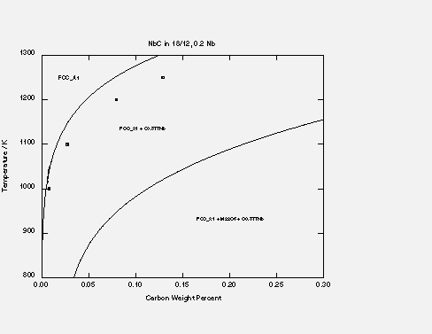
The picture below shows an isopleth of an 18Cr/12Ni steel with 0.2Nb. the first curve gives the solubility of carbon in austenite with regard to the niobium carbide of stoichiometry Nb:C 1:0.877. The curve is from mtdata, the points correspond to an empirical relationship found in literature, they have been added by editing the metafile.
| PT-group | 2003 Thomas Sourmail, Cambridge. | Please email feedback ! |