| (1) |
The development of chromium concentration profiles in austenitic stainless steels, due to the grain boundary precipitation of carbides has been modelled, taking account of multicomponent effects, both in the estimation of the state of equilibrium at the carbide/matrix interface and in diffusion. A comparison against published experimental data shows that the theory accounts for the development of the depleted zone as well as self-healing, unlike recent work where these effects are treated as separate phenomena. At the same time, the present model preserves local equilibrium at the precipitate-matrix interface and provides a natural explanation for the observation of delays in reaching the minimum chromium content.
| (1) |
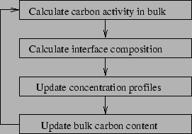
In steels, the interstitial-diffusion of carbon is much faster than
that of substitutional elements. It is therefore reasonable to assume
[3,4,5,6] that the activity of carbon in the
matrix becomes uniform, i.e, the activity at the carbide-matrix
interface equals far away from the interface. This is illustrated in
Figure 1. Such models predict a minimum chromium
concentration in the matrix at the carbide-matrix interface,
![]() reached at the beginning of precipitation
(t=0). As precipitation progresses, the activity of carbon decreases
and
reached at the beginning of precipitation
(t=0). As precipitation progresses, the activity of carbon decreases
and
![]() increases as required by local equilibrium
at the carbide-matrix interface.
increases as required by local equilibrium
at the carbide-matrix interface.
![\includegraphics[width=13cm,height=10.5cm]{figures/tie_line_p.eps}](img14.png)
|
Models by Stawström and Hillert [3], Was and Kruger [4], and Bruemmer [6] have applied this concept. With the restriction of a constant nickel content, Stawström and Hillert used a simple equation to calculate the carbon activity as a function of chromium and carbon. Was and Kruger introduced a more elaborate thermodynamic approach, accounting for Fe, Cr, Ni, C while Bruemmer added an empirical term to include the effect of Mo.
In these models, a knowledge of carbon isoactivity was used to
determine the chromium concentration at the interface. Assuming a
planar precipitate-matrix interface, the growth rate was then
estimated by solving the diffusion equation ahead of the interface. It
is worth noting that all of these models only allow for chromium
modification when estimating the carbide-matrix interface
composition. This is not strictly correct in systems with more than
three components such as the one dealt with by Was and Kruger, and
Bruemmer, since, for example there is no guarantee that the flux
balance equations:
| (2) | |||
| (3) |
As mentioned earlier, previous models
[3,4,5,6] implied that the
![]() is reached at t=0. However, measurements
[7] indicate that
is reached at t=0. However, measurements
[7] indicate that
![]() will only reach
a minimum after a finite time
will only reach
a minimum after a finite time ![]() as in Figure 2.
as in Figure 2.
![\includegraphics[width=7cm]{figures/crmindiagram.eps}](img19.png)
|
Sahlaoui et al. [8] recently developed a different
approach based on Mayo [9] where the process is divided into
two. Chromium-depletion is considered to occur during the growth of
the carbide according to an empirical equation:
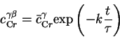 |
(4) |
The agreement achieved with experimental data by Sahlaoui et al.'s
model is essentially due to a fitting parameter ![]() in the first
stage of the calculation. Furthermore, the use of a two-stage
description violates the reasonable assumption that the carbide-matrix
interface should remain in local equilibrium during
diffusion-controlled growth. It will become evident later
in this paper that the predicted values of
in the first
stage of the calculation. Furthermore, the use of a two-stage
description violates the reasonable assumption that the carbide-matrix
interface should remain in local equilibrium during
diffusion-controlled growth. It will become evident later
in this paper that the predicted values of
![]() should underestimate experimental measurements which suffer from
spatial resolution problems. In the present work we hope to show that
the experimental data can be explained in a unified model consistent
with thermodynamic equilibrium.
should underestimate experimental measurements which suffer from
spatial resolution problems. In the present work we hope to show that
the experimental data can be explained in a unified model consistent
with thermodynamic equilibrium.
The mobilities were calculated as a function of the composition, as
suggested by Ågren and Åkermark [11,12].
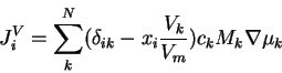
Practical calculations are made in the volume-fixed f.o.r. (for
example, Kirkaldy and Young [13]), defined
so that
![]() where Vi is the molar volume
of component i and JiV the flux of component i through a
surface of fixed coordinate in the volume-fixed f.o.r. Noting that:
where Vi is the molar volume
of component i and JiV the flux of component i through a
surface of fixed coordinate in the volume-fixed f.o.r. Noting that:
 |
(7) |
 |
(8) |
Using central difference for space and forward difference for time, the following finite-difference equivalent for equation 9 is obtained:
![\begin{displaymath}
\frac{x_{i}^{j,n+1}-x_{i}^{j,n}}{\Delta t} =
\frac{1}{(\Del...
...{ik}^{j-\frac{1}{2},n} (\mu_{k}^{j,n}-\mu_{k}^{j-1,n})
\right]
\end{displaymath}](img31.png) |
(10) |
 and
and
 can
be defined using:
can
be defined using:
| (12) |
The boundary conditions were set as follow:
| xij,0 | = | (13) | |
| xinmax,k | = | (14) |
| (15) |
The complexity of the task means that most models so far have limited
the search for the flux-balance to the Fe-Cr-C system (isoactivity
of carbon). An algorithm which uses MT-DATA has been written to solve
the problem in a general manner: not only is the isoactivity of carbon
satisfied, but the solution also verifies the flux balance for other
substitutional elements; for the example of a Fe-Cr-Ni-C system:
Table 1 provides the results obtained under different assumptions. In the first case, only Cr is modified to obtain carbon isoactivity. Clearly, the interface Ni content being below that of the bulk is not consistent with growth of the precipitate, since the latter has a lower Ni content. The second calculation satisfies both the isoactivity of carbon and equality of the Cr and Ni fluxes.
|
Note that at the interface, the flux is estimated using a forward spatial difference as it is not possible to define an ancillary node as is done for the last node in the bulk.
 |
When considering the amount of carbon removed from the matrix by the growth of the precipitate, it is necessary to define a volume from which the carbon is drawn. Stawström and Hillert [3] have used half the grain size for this purpose. This is discussed in detail later in the text.
| |||||||||||||||
Figure 4 compares the calculated
![]() as a function of temperature, against previous
work. Earlier approaches by Stawström and Hillert
[3], and Fullman [15] over-predicted
as a function of temperature, against previous
work. Earlier approaches by Stawström and Hillert
[3], and Fullman [15] over-predicted
![]() at high temperatures. Bruemmer [6]
applied an empirical relation which was obtained by direct
measurements of chromium-depletion. It is not therefore surprising
that Bruemmer's model is in good agreement with the measured data and
follow the trend of experimental data in which
at high temperatures. Bruemmer [6]
applied an empirical relation which was obtained by direct
measurements of chromium-depletion. It is not therefore surprising
that Bruemmer's model is in good agreement with the measured data and
follow the trend of experimental data in which
![]() increases with temperature.
increases with temperature.
Measurements of
![]() [7] were obtained
using a scanning transmission electron microscope with an energy
dispersive X-ray spectrometer (STEM-EDS) for which the beam
spreading was estimated to be
[7] were obtained
using a scanning transmission electron microscope with an energy
dispersive X-ray spectrometer (STEM-EDS) for which the beam
spreading was estimated to be ![]() 25 nm [7].
25 nm [7].
It is argued here that measurements are likely to overestimate the actual interface composition for two reasons: as is shown later, strong concentration gradients are expected in the vicinity of the grain boundary, meaning that the averaging effect caused by the beam spreading is likely to have a significant influence on the result. Furthermore, the problem of having a grain boundary parallel to the beam is never mentioned in the experimental procedure, although having to satisfy both this condition and the tilt required by the detector geometry is certainly a source of experimental difficulties.
There are therefore good reasons to believe that the measured
`interface' composition is best compared with the average composition
of the first ![]() 25 nm of material in contact with the grain
boundary.
25 nm of material in contact with the grain
boundary.
![\includegraphics[width=10cm]{figures/averages.eps}](img51.png)
|
Figure 5 shows the evolution of the average weight
fraction of chromium in the first 15, 20 and 25 nm, for a 18.48 Cr,
8.75 Ni, 0.06 C (wt%) steel aged at 700 ![]() C. The relatively small
influence in the distance over which the average is calculated is to
be expected. If on the contrary, a strong dependency had been shown
over this range, the literature would surely provide significantly
different measurements depending on the exact experimental conditions;
this does not seem to be the case. In the discussion that follows, the
interface value is referred to as
C. The relatively small
influence in the distance over which the average is calculated is to
be expected. If on the contrary, a strong dependency had been shown
over this range, the literature would surely provide significantly
different measurements depending on the exact experimental conditions;
this does not seem to be the case. In the discussion that follows, the
interface value is referred to as
![]() , and the averaged
value calculated over the first 25 nm as
, and the averaged
value calculated over the first 25 nm as
![]() .
.
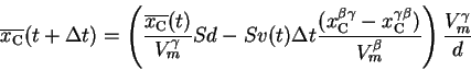
The self-healing process, on the other hand, is due to the shift of the tie-line towards the mass-balance equilibrium as the precipitation progresses, as illustrated in Figure 6. The time scale in which this phenomenon occurs is strongly dependent on the volume (V=Sd) from which carbon is withdrawn. S is set to be a unit area, and d is the distance ahead of the grain boundary from which carbon can be drawn. For a small d, the carbon concentration is expected to drop rapidly and self-healing should start relatively early (Figure 7).
At the limit where the distance d is infinite, the activity of carbon in
the bulk is constant and self-healing never occurs. For very small
d, sensitisation can be avoided as the increase of Cr concentration
at the interface is fast enough so that the average in the first 25 nm
never drops below a critical value. This has been observed
experimentally by Beltran et al.[16]: with a grain size of
15 ![]() m, sensitisation was found to be virtually reduced to zero throughout
the ageing while a far greater effect is observed for a grain size of
150
m, sensitisation was found to be virtually reduced to zero throughout
the ageing while a far greater effect is observed for a grain size of
150 ![]() m. The relation between d and the grain size,
overlooked in many previous works, is discussed later.
m. The relation between d and the grain size,
overlooked in many previous works, is discussed later.
![\includegraphics[width=10cm]{figures/carbon_depletion.eps}](img55.png)
|
The evolution of the carbon mole fraction in the bulk is calculated
according to:
Figure 8(a) shows predicted chromium
concentration profiles ahead of the grain boundary for identical
temperatures and ageing durations, for a variety of values of d.
In all cases, the interface chromium mole fraction at t=0 is
identical. After 100 h, significant tie-line shifting has occurred for
the smallest d but virtually none for the largest
d. Figure 8(b) shows the average
chromium mole fraction (
![]() )
over the first 25 nm in the different cases.
Note that for a small value of d, the minimum of
)
over the first 25 nm in the different cases.
Note that for a small value of d, the minimum of
![]() is about 4
wt% higher than the minimum interface value (at t=0) while this
difference is reduced to 1 wt% for d=5
is about 4
wt% higher than the minimum interface value (at t=0) while this
difference is reduced to 1 wt% for d=5 ![]() m.
m.
![\includegraphics[height=55mm]{figures/profiles.eps}](img61.png)
![\includegraphics[height=55mm]{figures/distance.eps}](img62.png)
|
One of the difficulties occurring in physical models is to establish a
correspondence between the predicted evolution of the concentrations
and the sensitisation phenomenon itself. A criterion could be that
sensitisation starts when
![]() is below a
critical value, and ends when it raises above this value.
is below a
critical value, and ends when it raises above this value.
As illustrated in Figure 8(b), the onset of sensitisation is relatively independent on d. Prediction of desensitisation is less successful (Figure 9); possible reasons are discussed later.
![\includegraphics[height=60mm]{figures/stawstrom.eps}](img64.png)
|
Stawström and Hillert [3] have used half the grain size for d. However, the real soft-impingement being a three-dimension problem, it seems more appropriate to attribute to each calculation volume a sixth of the grain, given that, if a simple cubic model is used to represent a grain, six faces will actually draw carbon from the same volume.
If, as with Stawström and Hillert [3], a distance of
25 ![]() m is used, a film
of about 0.25
m is used, a film
of about 0.25 ![]() m on each side of the boundary, is required to
obtain the average 1% volume fraction of M23C6 found in type 304 at
700
m on each side of the boundary, is required to
obtain the average 1% volume fraction of M23C6 found in type 304 at
700![]() C. This is significantly larger than the typical 200 nm
[7] observed as a maximum thickness (meaning that the
equivalent film of uniform thickness would be thinner).
C. This is significantly larger than the typical 200 nm
[7] observed as a maximum thickness (meaning that the
equivalent film of uniform thickness would be thinner).
In the present model, desensitisation times are still slightly overestimated even if d is set to a sixth of the grain size (Figure 9).
All of the models for sensitisation
[3,4,7,9,8],
only consider grain-boundary precipitation, which
always happen at the very early stage of ageing. This can be
sufficient, as illustrated previously, to predict the onset of
sensitisation. However, desensitisation occurs on longer time scale
where other carbon sinks becomes active within the grain.
In particular, Lewis and Hattersley [17] reported
observing intragranular M23C6 as early as after 30 minutes at
750 ![]() C, after a few hundred hours, the quantity of
intragranular M23C6 is significant ().
The consequences may not be negligible in steels with relatively large
grain sizes.
C, after a few hundred hours, the quantity of
intragranular M23C6 is significant ().
The consequences may not be negligible in steels with relatively large
grain sizes.
![\includegraphics[height=65mm]{figures/ttp_m23c6.eps}](img65.png)
|
To verify whether the shorter than predicted self-healing times could
be attributed to intragranular precipitation, a simple modification
was made to the existing model, under the following assumptions:
intragranular particles of M23C6 form on dislocations, on which
nucleation is taken to be instantaneous. Note that this is not
unreasonable given the identification of intragranular M23C6 after 30
minutes at 750 ![]() C [17].
C [17].
Assuming a spherical shape, the volume increment during a time step
is given by:
| (19) |
![\includegraphics[height=70mm]{./figures/N_effect_650C.eps}](img67.png)
|
The role of intragranular precipitation is also dependent on the grain size, as illustrated in Figure 12, which shows that, for N=1023 m-3, the desensitisation time is significantly shifted to the left.
Figure 12 illustrates the estimated influence of intragranular
precipitation on a material of two different grain sizes, 50 and 150
![]() m, at 650
m, at 650 ![]() C and 700
C and 700 ![]() C. As is expected, precipitation
within the grain has no influence on the onset of sensitisation but
can strongly affect the predicted self-healing as the grain size
increases and the amount of surface per unit volume is reduced.
C. As is expected, precipitation
within the grain has no influence on the onset of sensitisation but
can strongly affect the predicted self-healing as the grain size
increases and the amount of surface per unit volume is reduced.
![\includegraphics[height=50mm]{./figures/650_and_700_50mu.eps}](img68.png)
![\includegraphics[height=50mm]{./figures/150mum.eps}](img69.png)
|
It should be noted that, by contrast with many former approaches, there are here no fitting parameters (e.g. [8]), or modifications of the thermodynamics for M23C6 formation (e.g. [6]), as the general SGTE database is used through MT-DATA. It is shown, first, that there is no need to modify these thermodynamic data to explain the measured Cr minimum, which, it is argued, should be under-predicted; and second, that the division of the sensitisation process in a two-stage process (e.g. [8], [9]) is not required to explain the delay in the observation of a Cr minimum near the grain boundaries.
The present model, consistent with experimental observations, predicts a delay in reaching a minimum interface chromium concentration at a small distance away from the carbide-matrix interface whilst maintaining the local equilibrium at the interface. It is also shown that the effect of intragranular precipitation on desensitisation cannot be neglected when considering large grain sizes.
This document was generated using the LaTeX2HTML translator Version 2002 (1.62)
Copyright © 1993, 1994, 1995, 1996,
Nikos Drakos,
Computer Based Learning Unit, University of Leeds.
Copyright © 1997, 1998, 1999,
Ross Moore,
Mathematics Department, Macquarie University, Sydney.
The command line arguments were:
latex2html -split 1 -title 'Sensitisation and Evolution of Chromium-depleted Zones in Fe-Cr-Ni-C systems.' -noparbox_images -math_parsing -notop_navigation -nonavigation submitted.tex
The translation was initiated by on 2003-07-02
![\begin{displaymath}
x_{i}^{j,n+1}
= x_{i}^{j,n} + \frac{\Delta t}{(\Delta X)^{2}...
...{ik}^{j-\frac{1}{2},n} (\mu_{k}^{j,n}-\mu_{k}^{j-1,n})
\right]
\end{displaymath}](img32.png)
![\includegraphics[width=8cm]{figures/result1.eps}](img49.png)
![\includegraphics[width=80mm]{figures/rslt_tieline.eps}](img54.png)