Materials Science and Technology, 21 (2005) 1293-1302.
Download PDF file of paper together with other information.
H. K. D. H. Bhadeshia
University of Cambridge
Materials Science and Metallurgy
Pembroke Street, Cambridge CB2 3QZ, U. K.
www.phase-trans.msm.cam.ac.uk
Most new materials are introduced by selectively comparing their properties against those of steels. Steels set this standard because iron and its alloys have so much potential that new concepts are discovered and implemented with notorious regularity.
In this 52nd Hatfield Memorial Lecture, I describe a remarkably beautiful microstructure consisting of slender crystals of ferrite, whose controlling scale compares well with that of carbon nanotubes. The crystals are generated by the partial transformation of austenite, resulting in an extraordinary combination of strength, hardness and toughness. All this in bulk steel without the use of expensive alloying elements. We now have a strong alloy of iron, which can be used for making items which are large in all three dimensions, which can be made without the need for mechanical processing or rapid cooling and which is cheap to produce and apply.
It is possible to think of many ways of creating extremely strong materials. Polycrystalline metals can be strengthened by reducing the scale of the microstructure whereas single crystals benefit from perfection. Carbon-based materials can in principle become incredibly strong if the only mode of deformation involves the stretching of carbon-carbon covalent bonds. These and many other mechanisms of strengthening unfortunately have limitations. In particular, it is difficult to make strong, isotropic materials which can be used to manufacture large components of arbitrary shape, whilst maintaining an attractive combination of properties at a reasonable cost. Such a material would be commercially viable over a broad range of applications.
Imagine in this context, a steel which is exceedingly strong, that can be made in large chunks, one which is easy to manufacture, and has a cost which is affordable. Before describing this novel material, it is important to review the meaning of strength, for there are many promises in the modern scientific and popular literature of materials which possess strength beyond our dreams. I shall attempt in this lecture to make appropriate comparisons to show how steels feature in this scenario.
The strength of crystals increases sharply as they are made smaller [1,2,3,4,5,6,7]. This is because the chances of avoiding defects become greater as the volume of the sample decreases. In the case of metals, imperfections in the form of dislocations are able to facilitate shear at much lower stresses than would be the case if whole planes of atoms had to collectively slide across each other [8,9]. Since defects are very diffcult to avoid, the strength in the absence of defects is said to be that of an ideal crystal.
In an ideal crystal, the tensile strength ![]() where
where ![]() is the
Young's modulus. The corresponding ideal shear strength is
is the
Young's modulus. The corresponding ideal shear strength is ![]() , where
, where ![]() is the shear modulus,
is the shear modulus, ![]() is a repeat period along the displacement direction and
is a repeat period along the displacement direction and ![]() is the spacing of the slip planes [8]. For ferritic iron,
is the spacing of the slip planes [8]. For ferritic iron, ![]() GPa and
GPa and ![]() GPa [10]. It
follows that the ideal values of tensile and shear strength should be about 21 GPa and 11 GPa respectively. In fact, tensile strengths approaching the theoretical values were achieved by
Brenner as long ago as 1956 (Fig. 1a) during the testing of whiskers of iron with diameters less than 2
GPa [10]. It
follows that the ideal values of tensile and shear strength should be about 21 GPa and 11 GPa respectively. In fact, tensile strengths approaching the theoretical values were achieved by
Brenner as long ago as 1956 (Fig. 1a) during the testing of whiskers of iron with diameters less than 2 ![]() m [5,7]. It is interesting that these stress levels fall out of the regime where Hooke's law
applies (Fig. 1b).
m [5,7]. It is interesting that these stress levels fall out of the regime where Hooke's law
applies (Fig. 1b).
|
(a)
![\includegraphics[width=7.0cm]{Figures/Brenner.strength.eps}](img14.png) (b) (b) ![\includegraphics[width=8.0cm]{Figures/Brenner.elastic.eps}](img15.png) |
The strength decreased sharply as the dimensions of the whiskers were increased (Fig. 1a), because of ``defects which are distributed statistically in a rather complex manner" [5,7]. It was therefore recognised many decades ago that it is not wise to rely on perfection as a method of designing strong materials, although it remains the case that incredible strength can be achieved by reducing dimensions, in the case of iron, to a micrometer scale. It is in this context that we now proceed to examine claims that large scale engineering structures can be designed using long carbon-nanotubes [11,12].
The existence of single-walled carbon tubes was pointed out in 1976 [13] but the subject seems to have become prominent after the discovery of ![]() in 1985 [14] and the identification of nanotubes by Iijima in 1991 [15]. These tubes can be imagined to be constructed from sheets of graphene consisting of sp
in 1985 [14] and the identification of nanotubes by Iijima in 1991 [15]. These tubes can be imagined to be constructed from sheets of graphene consisting of sp![]() carbon arranged in a two-dimensional hexagonal lattice (Fig. 2, [16]). The sheets, when rolled up and with the butting edges
appropriately bonded, are the nanotubes, which may or may not be capped by fullerne hemispheres. This is a simplified picture - it is well known that the actual form can be complex, for example with
occasional pentagonal rings of carbon atoms instead of hexagonal to accommodate changes in shape [17].
carbon arranged in a two-dimensional hexagonal lattice (Fig. 2, [16]). The sheets, when rolled up and with the butting edges
appropriately bonded, are the nanotubes, which may or may not be capped by fullerne hemispheres. This is a simplified picture - it is well known that the actual form can be complex, for example with
occasional pentagonal rings of carbon atoms instead of hexagonal to accommodate changes in shape [17].
|
(a)
![\includegraphics[width=8.0cm]{Figures/graphene.eps}](img18.png) (b) (b) ![\includegraphics[width=7.0cm]{Figures/graphene.nanotube.eps}](img19.png) |
The carbon-carbon chemical bond in a graphene layer may be the strongest bond in an extended system [18]; carbon is also light, so it is not surprising that
there are numerous papers which talk about the potential of long carbon-nanotubes as engineering materials which rival steel. The modulus of these tubes along the axis is about 1.28![]() TPa [18], comparable to that of diamond [19].
TPa [18], comparable to that of diamond [19].
The calculated breaking strength of such a tube has been estimated to be 130 GPa [20]; this number is so astonishing that it has led to many exaggerated statements which are frequently repeated and hence have taken the form of ``truth" in the published literature. For example, the tubes are said to be a hundred times stronger than steel; we have seen that whiskers of iron which are much bigger than carbon nanotubes, achieve a strength which is 14 GPa, with the potential of reaching 21 GPa.
There are in the literature, bizarre statements which take no account of defects. For example, it is said that a ``macroscopic one-inch thick rope, where 1014 parallel buckywires (nanotube ropes) are all holding together" will be as strong as theory predicts, i.e. 130 GPa [22].
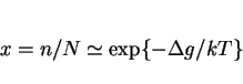
What all of this ignores is that materials will contain defects![]() . Some of these defects will be there at equilibrium, i.e., they cannot be avoided. For example, it is known that metals contain an
equilibrium concentration of vacancies. The enthalpy change associated with the formation of a vacancy opposes its existence, whereas the change in configurational entropy due to the formation
of a vacancy favours its formation. The total change in free energy on forming
. Some of these defects will be there at equilibrium, i.e., they cannot be avoided. For example, it is known that metals contain an
equilibrium concentration of vacancies. The enthalpy change associated with the formation of a vacancy opposes its existence, whereas the change in configurational entropy due to the formation
of a vacancy favours its formation. The total change in free energy on forming ![]() vacancies in a crystal is given by
[24]:
vacancies in a crystal is given by
[24]:
Edwards [11] has estimated that 120,000 km gigatubes grown with the properties of carbon nanotubes are needed to construct a space elevator. He further
estimates that such a cable would weigh around 5000 kg. Based on this, assuming an upper limit of ![]() eV [20], and neglecting dimensionality differences,
equation 2 can be used to calculate the equilibrium number of monovacancies expected as a function of temperature, Fig.
3. In this, the temperature of interest is that at which the carbon is assembled; this can typically range from 2000-4000 K, giving a large number of equilibrium defects. Given that the
actual value of
eV [20], and neglecting dimensionality differences,
equation 2 can be used to calculate the equilibrium number of monovacancies expected as a function of temperature, Fig.
3. In this, the temperature of interest is that at which the carbon is assembled; this can typically range from 2000-4000 K, giving a large number of equilibrium defects. Given that the
actual value of ![]() is much smaller than the 7 eV for a flat graphene sheet [20], it cannot ever be assumed that defect-free gigatubes can be made with properties approaching tubes which are some 18 orders of magnitude smaller.
is much smaller than the 7 eV for a flat graphene sheet [20], it cannot ever be assumed that defect-free gigatubes can be made with properties approaching tubes which are some 18 orders of magnitude smaller.
|
(a)
![\includegraphics[width=9.5cm]{Figures/elevator.eps}](img34.png) (b) ![\includegraphics[width=12cm]{Figures/vacancies.eps}](img35.png) |
Statement 1: Systems which rely on perfection in order to achieve strength necessarily fail on scaling to engineering dimensions. Indeed, there is no carbon tube which can match the strength of iron beyond a scale of 2 mm.
Although we have considered here vacancies and made many assumptions in the estimation of defect density, the fact that the measured strengths of nanotubes as shown in Table 1 are frequently much smaller than expected from vacancy models [21] indicates the presence of more severe defects in the atomic structure of the tubes.
|
Suppose that gigatubes of carbon could be made capable of supporting a stress of 130 GPa. Would this allow for safe engineering design? One aspect of safe design is that fast fracture should
be avoided; most metals absorb energy in the form of plastic deformation before ultimate fracture. Energy absorption in an accident is a key aspect of automobile safety. Carbon nanotubes are not in
this sense defect tolerant; their deformation prior to fracture is elastic. The stored energy density in a tube stressed to 130 GPa, given an elastic modulus along its length of ![]() 1.2 TPa is in excess of that associated with dynamite, Table 2. Dynamite is explosive
because of its high energy density and because this energy is released rapidly, the detonation front propagating at some 6000 m
1.2 TPa is in excess of that associated with dynamite, Table 2. Dynamite is explosive
because of its high energy density and because this energy is released rapidly, the detonation front propagating at some 6000 m![]() s
s![]() . The speed of an elastic wave in the carbon is given by
. The speed of an elastic wave in the carbon is given by ![]() where
where ![]() is the density. In the event of
fracture, the rate at which the stored energy would be released is much greater than that of dynamite (Table 2), meaning that fracture is unlikely to occur in
a safe manner.
is the density. In the event of
fracture, the rate at which the stored energy would be released is much greater than that of dynamite (Table 2), meaning that fracture is unlikely to occur in
a safe manner.
| J g |
m s |
|
| Dynamite | 4650 | 6000 |
| Carbon nanotube | 5420 | 21500 |
iStatement 2: Structures in tension, which reversibly store energy far in excess of their ability to do work during fracture must be regarded as unsafe.
It has been possible for some time to obtain commercially, steel wire which has an ultimate tensile strength of 5.5 GPa and yet is very ductile in fracture [29,30,31]. Scifer, as the wire is known, is made by drawing a dual-phase microstructure of martensite
and ferrite in Fe-0.2C-0.8Si-1Mn wt% steel in the form of 10 mm diameter rods, into strands which individually have a diameter of about 8 ![]() m. This amounts to a huge deformation with a true strain in excess of 9. The dislocation cell size in the material becomes about 10-15 nm in size (Fig. 4a). This is where much of the strength of Scifer comes from [30,31]. A similar stainless
steel thread is also available commercially [32].
m. This amounts to a huge deformation with a true strain in excess of 9. The dislocation cell size in the material becomes about 10-15 nm in size (Fig. 4a). This is where much of the strength of Scifer comes from [30,31]. A similar stainless
steel thread is also available commercially [32].
The fact that the properties are here achieved by introducing defects, also means that the strength of Scifer is insensitive to its size as shown in Fig. 4b.
|
(a)
![\includegraphics[width=7.5cm]{Figures/scifer.probe.eps}](img41.png) (b) (b) ![\includegraphics[width=7.5cm]{Figures/scifer1.eps}](img42.png) (c) (c) ![\includegraphics[width=6.5cm]{Figures/denier.eps}](img43.png) |
A denier is the weight in grams of 9 km of fibre or yarn. A 50 denier thread is typically used in making socks whereas stockings are made from 10 denier fibre. Scifer is just 9 denier in this classification; this highlights one of the difficulties in using deformation to increase strength. The deformation necessary to accumulate a large number density of defects limits the size and form of the product, in the case of Scifer to that of a textile thread. Deformation processes such as equichannel angular processing [33,34] and accumulative roll-bonding [35,36] maintain the overall dimensions but the range of shapes that can be achieved is limited.
Statement 3: The properties of severely deformed materials are insensitive to size but the forms that can be produced are limited.
High-strength low-alloy steels produced using thermomechanical processing have been described as one of the wonders of the world [37]. They have contributed so
much to the quality of engineered products that tens of billions of tonnes of such alloys now permeate all aspects of life. During the processing, fine austenite ![]() grains are generated by a combination of deformation and recrystallisation; the austenite finally transforms into fine grains of ferrite
grains are generated by a combination of deformation and recrystallisation; the austenite finally transforms into fine grains of ferrite ![]() , with a size typically of 10
, with a size typically of 10![]() m. The recent search has been for processes which reduce the grain size dramatically to less than 1
m. The recent search has been for processes which reduce the grain size dramatically to less than 1 ![]() m [38,39,40]. Fine grains represent one of the few mechanisms available to increase both
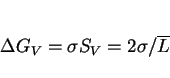
strength and toughness. What then is the theoretical minimum grain size that can be achieved using this technology? This question can be answered by noting that the excess energy stored in the form
of grain boundaries cannot exceed the free energy change
m [38,39,40]. Fine grains represent one of the few mechanisms available to increase both
strength and toughness. What then is the theoretical minimum grain size that can be achieved using this technology? This question can be answered by noting that the excess energy stored in the form
of grain boundaries cannot exceed the free energy change ![]() due to the transformation of the austenite [41].
due to the transformation of the austenite [41].
For an equiaxed polycrystalline grain structure, the grain boundary surface per unit volume (![]() ) is related to the
grain size
) is related to the
grain size ![]() (mean lineal intercept) by the equation
(mean lineal intercept) by the equation ![]() . The stored energy per unit volume due to the grain boundaries is then
. The stored energy per unit volume due to the grain boundaries is then
 |
(4) |
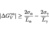
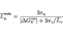
Figure 5 shows the variation in the limiting ferrite grain size ![]() as a function of
as a function of ![]() , calculated using equation 5 with
, calculated using equation 5 with ![]() Jm
Jm![]() ; given
the absence of data the
; given
the absence of data the ![]() term in equation 6 was set to zero. These
calculations are presented as the `ideal' curve in figure 5. The curve indicates that at large grain sizes,
term in equation 6 was set to zero. These
calculations are presented as the `ideal' curve in figure 5. The curve indicates that at large grain sizes, ![]() is sensitive to
is sensitive to ![]() and hence to the undercooling below the equilibrium transformation temperature. However, reductions in grain size in the submicrometre range require huge values of
and hence to the undercooling below the equilibrium transformation temperature. However, reductions in grain size in the submicrometre range require huge values of ![]() , meaning that the transformations would have to be suppressed to large undercoolings to achieve fine grain size.
, meaning that the transformations would have to be suppressed to large undercoolings to achieve fine grain size.
![\includegraphics[width=12cm]{Figures/ferrite.eps}](img64.png) |
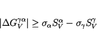
Also plotted on Fig. 5 are points corresponding to measured ferrite grain sizes from the low and high-Mn steels as described elsewhere [41]; It is evident that except at the lowest undercoolings, ![]() . The data indicate that in spite of tremendous efforts, the
smallest ferrite grain size obtained commercially using thermomechanical processing is stuck at about 1
. The data indicate that in spite of tremendous efforts, the
smallest ferrite grain size obtained commercially using thermomechanical processing is stuck at about 1 ![]() m.
m.
The reason for this is recalescence, which is the heating of the sample caused by release of the latent heat of transformation at a rate which is so high that it cannot easily be dissipated by diffusion. This rise in temperature due to recalescence reduces the effective undercooling and hence the driving force for transformation [41]. It is seen from Fig. 5 that the recalescence-corrected curves show better agreement with the experimental data, indicating that at large undercoolings, the achievement of fine grain size is limited by the need to dissipate enthalpy during rapid transformation.
To achieve submicrometre grain sizes it is necessary to transform at large undercoolings, but the rate of transformation then increases, leading to recalescence, which defeats the objective. Large
scale thermomechanical processing is therefore limited by recalescence and it is unlikely to lead to grain sizes which are uniformly less than about 1 ![]() m.
m.
Statement 4: To achieve submicrometre grain sizes it is necessary to transform at large undercoolings, but the rate of transformation then increases, leading to recalescence, which defeats
the objective. Large scale thermomechanical processing is therefore limited by recalescence and is unlikely to lead to grain sizes which are uniformly less than about 1 ![]() m.
m.
Very strong martensitic steels with strength greater than 3 GPa already exist [42]. This kind of martensite is produced in fairly large steel samples by rapid cooling from the austenitic condition. However, the dimensions can be limited by the need to achieve a uniform microstructure, a fact implicit in the original concept of hardenability. To increase hardenability requires the addition of expensive alloying elements. The rapid cooling can lead to undesirable residual stresses [43,44] which can ruin critical components and which have to be accounted for in component-life assessments.
It would be nice to have a strong material which can be used for making components which are large in all their dimensions, and which does not require mechanical processing or rapid cooling to reach the desired properties. We have seen that the following conditions are required to achieve this:
Steel transformed into carbide-free bainite can satisfy these criteria. Bainite and martensite are generated from austenite without diffusion by a displacive mechanism. Not only does this lead to solute-trapping but also a huge strain energy term, both of which reduce the heat of transformation [45,46,47]. The growth of individual plates in both of these transformations is fast, but unlike martensite, the overall rate of reaction is much smaller for bainite. This is because the transformation propagates by a sub-unit mechanism in which the rate is controlled by nucleation rather than growth [48]. This mitigates recalescence.
Suppose we now attempt to calculate the lowest temperature at which bainite can be induced to grow. We have the theory to address this proposition [49,50,51,52,53]. Such calculations are illustrated in Figure 6a, which shows for an example steel, how the bainite-start (![]() ) and martensite-start
(
) and martensite-start
(![]() ) temperatures vary as a function of the carbon concentration. There is in principle no lower limit to the
temperature at which bainite can be generated. On the other hand, the rate at which bainite forms slows down drastically as the transformation temperature is reduced, as shown by the calculations in
Figure 6b. It may take hundreds or thousands of years to generate bainite at room temperature. For practical purposes, a transformation time of tens of days
is reasonable. But why bother to produce bainite at a low temperature?
) temperatures vary as a function of the carbon concentration. There is in principle no lower limit to the
temperature at which bainite can be generated. On the other hand, the rate at which bainite forms slows down drastically as the transformation temperature is reduced, as shown by the calculations in
Figure 6b. It may take hundreds or thousands of years to generate bainite at room temperature. For practical purposes, a transformation time of tens of days
is reasonable. But why bother to produce bainite at a low temperature?
![\includegraphics[width=15cm]{Figures/Figure1.eps}](img67.png) |
Experiments consistent with the calculations illustrated in Figure 6 demonstrated that in a Fe-1.5Si-2Mn-1C wt% steel (detailed composition in
Table 3), bainite can be generated at a temperature as low at 125![]() C [56],
which is so low that the diffusion distance of an iron atom is an inconceivable 10
C [56],
which is so low that the diffusion distance of an iron atom is an inconceivable 10![]() m over the time scale of the
experiment!
m over the time scale of the
experiment!
What is even more remarkable is that the plates of bainite are only 20-40 nm thick. The slender plates of bainite are dispersed in stable carbon-enriched austenite which, with its face-centred cubic lattice, buffers the propagation of cracks. The optical and transmission electron microstructures are shown in Fig. 7; they not only have metallurgical significance in that they confirm calculations, but also are elegant to look at. Indeed, the microstructure has now been characterised, both chemically and spatially to an atomic resolution; the pleasing aesthetic appearance is maintained at all resolutions. There is no redistribution of substitutional atoms on the finest conceivable scale [57].
![\includegraphics[width=12cm]{Figures/Figure2a.eps}](img69.png) ![\includegraphics[width=12cm]{Figures/Figure2b.eps}](img70.png) |
Ultimate tensile strengths of 2500 MPa in tension have routinely been obtained, ductilities in the range 5-30% and toughness in excess of 30-40 ![]() . All this in a dirty steel which has been prepared ordinarily and hence contains inclusions
and pores which would not be there when the steel is made by any respectable process. The bainite is also the hardest ever achieved, 700 HV [56]. The simple heat
treatment involves the austenitisation of a chunk of steel (at say 950
. All this in a dirty steel which has been prepared ordinarily and hence contains inclusions
and pores which would not be there when the steel is made by any respectable process. The bainite is also the hardest ever achieved, 700 HV [56]. The simple heat
treatment involves the austenitisation of a chunk of steel (at say 950![]() C), gently transferring into an oven at
the low temperature (at say 200
C), gently transferring into an oven at
the low temperature (at say 200![]() C) and holding there for ten days or so to generate the microstructure. There is
no rapid cooling - residual stresses are avoided. The size of the sample can be large because the time taken to reach 200
C) and holding there for ten days or so to generate the microstructure. There is
no rapid cooling - residual stresses are avoided. The size of the sample can be large because the time taken to reach 200![]() C from the austenitisation temperature is much less than that required to initiate bainite. Our tests indicate uniform microstructure in 80 mm thick samples - thicker samples were
not available but calculations indicate that dimensions greater than 200 mm will show similar results. This is a major commercial advantage [60].
C from the austenitisation temperature is much less than that required to initiate bainite. Our tests indicate uniform microstructure in 80 mm thick samples - thicker samples were
not available but calculations indicate that dimensions greater than 200 mm will show similar results. This is a major commercial advantage [60].
It is cheap to heat-treat something at temperatures where pizzas are normally cooked. But suppose there is a need for a more rapid process. The transformation can easily be accelerated to occur within hours, by adding solutes which decrease the stability of austenite. Aluminium and cobalt, in concentrations less than 2 wt%, have been shown to accelerate the transformation in the manner described. Both are effective, either on their own or in combination [61].
|
Much of the strength and hardness of the microstructure comes from the very small thickness of the bainite plates. Of the total strength of 2500 MPa, some 1600 MPa can be attributed solely to the fineness of the plates. The residue of strength comes from dislocation forests, the strength of the iron lattice and the resistance to dislocation motion due to solute atoms. Because there are many defects created during the growth of the bainite [46], a large concentration of carbon remains trapped in the bainitic ferrite and does not precipitate, probably because it is trapped at defects [65].
Whereas the ordinary tensile strength of the strong bainite is about 2.5 GPa, the strength has been reported to be as high as 10 GPa at the very high strain rates ( ![]() ) associated with ballistic tests illustrated in Fig.
8 [66]. The strong bainite has therefore found application in armour [67,68].
Fig. 9 shows a series of tests conducted using projectiles which are said to involve ``the more serious battlefield tests" (the details are proprietary).
Figs. 9a,b show experiments in which an armour system is tested. A 12 mm thick sample of the bainitic steel is sandwiched between vehicle steel,
the whole contained in glass-reinforced plastic. In ordinary armour the projectile would have penetrated completely whereas the bainite has prevented this; the steel did however crack. By reducing
the hardness (transforming at a higher temperature), it was possible for the armour to support multiple hits (Fig. 9c) without being incorporated in an
armour-system.
) associated with ballistic tests illustrated in Fig.
8 [66]. The strong bainite has therefore found application in armour [67,68].
Fig. 9 shows a series of tests conducted using projectiles which are said to involve ``the more serious battlefield tests" (the details are proprietary).
Figs. 9a,b show experiments in which an armour system is tested. A 12 mm thick sample of the bainitic steel is sandwiched between vehicle steel,
the whole contained in glass-reinforced plastic. In ordinary armour the projectile would have penetrated completely whereas the bainite has prevented this; the steel did however crack. By reducing
the hardness (transforming at a higher temperature), it was possible for the armour to support multiple hits (Fig. 9c) without being incorporated in an
armour-system.
![\includegraphics[width=9cm]{Figures/hammond.eps}](img73.png) |
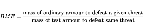
The ballistic mass efficiency BME of an armour is defined as
 |
(7) |
|
(a)
![\includegraphics[width=5cm]{Figures/armour1.eps}](img75.png) (b) (b) ![\includegraphics[width=5cm]{Figures/armour2.eps}](img76.png) (c) ![\includegraphics[width=5cm]{Figures/armour3.eps}](img77.png) (d) (d) ![\includegraphics[width=8cm]{Figures/armour4.eps}](img78.png) |
High-carbon steels are difficult to weld because of the formation of untempered, brittle martensite in the coarse-grained heat-affected zones of the joints. The martensite fractures easily, leading to a gross deterioration in the structural integrity of the joint. For this reason, the vast majority of weldable steels have low carbon concentrations. It would be desirable therefore to make the low-temperature bainite with a much reduced carbon concentration.
|
(a)
![\includegraphics[width=6.5cm]{Figures/BSMS1.eps}](img79.png) (b) (b) ![\includegraphics[width=6.5cm]{Figures/BSMS2.eps}](img80.png) |
Calculations done using the scheme outlined elsewhere [49,69] indicate that carbon is much more effective in maintaining a
difference between the ![]() and
and ![]() temperatures than are substitutional solutes which reduce
temperatures than are substitutional solutes which reduce ![]() simultaneously for martensite and bainite, Fig. 10. Substitutional solutes do not partition during any stage in the formation of martensite or bainite; both transformations are therefore identically affected by the way in
which the substitutional solute alters the thermodynamic driving force. It is the partitioning of carbon at the nucleation stage which is one of the distinguishing features of bainite when compared
with martensite. This carbon partitioning allows bainite to form at a higher temperature than martensite. This advantage is diminished as the overall carbon concentration is reduced, as illustrated
in Figure 10.
simultaneously for martensite and bainite, Fig. 10. Substitutional solutes do not partition during any stage in the formation of martensite or bainite; both transformations are therefore identically affected by the way in
which the substitutional solute alters the thermodynamic driving force. It is the partitioning of carbon at the nucleation stage which is one of the distinguishing features of bainite when compared
with martensite. This carbon partitioning allows bainite to form at a higher temperature than martensite. This advantage is diminished as the overall carbon concentration is reduced, as illustrated
in Figure 10.
From these results, it must be concluded that it is not possible to design low-temperature bainite with a low carbon concentration.
The ultimate focus of this lecture has been the ability to make large chunks of strong and tough steel. But it has been necessary to place this in the wider context of strong materials in order to allow sensible comparisons to be made.
When claims are made about strong materials for structural applications, they seem frequently to neglect the elementary science of scale. Just because it is possible to produce a nanotube of carbon which has a calculated strength of 130 GPa and a measured strength approaching that value, it does not mean that this can be translated into a fibre of a length visible to the naked eye, let alone the 120,000 km needed to begin thinking about a space-elevator. Indeed, it may not be possible even in principle to scale the properties given the existence of entropy-stabilised equilibrium defects.
It is noticeable in the contemporary materials literature that strength is a term which is much abused. It is common to claim that a novel material is as strong as steel, without specifying the nature of the steel against which the comparison is made. The claimants are either ignorant of the fact that it is possible to commercially make polycrystalline iron with a strength as low as 50 MPa or as high as 5.5 GPa, or neglect it to impress a fickle audience. In an academic context, single crystals of iron have been made which behave elastically to a stress of 14 GPa, taking them into a range of recoverable strain where Hooke's law does not apply.
Statement 5: The bainite obtained by transformation at very low temperatures is the hardest ever, has considerable ductility (almost all of it uniform), does not require mechanical
processing, does not require rapid cooling, the steel after heat-treatment therefore does not have long-range residual stresses, it is very cheap to produce and has uniform properties in very large
sections. In effect, the hard bainite has achieved all of the essential objectives of structural nanomaterials which are the subject of so much research![]() BUT IN LARGE CHUNKS!
BUT IN LARGE CHUNKS!
There remain, as is always the case, many parameters which have yet to be characterised, for example the fatigue and stress-corrosion properties.
I am grateful to M. Endo for providing the images of the graphene and the schematic illustration of the graphene to nanotube transition. It is an especial pleasure to acknowledge Francisca Garcia Caballero for the original work on hard bainite. I would also like to thank Carlos Garcia Mateo, Mathew Peet, Kazu Hase, Suresh Babu, Mike Miller, Peter Brown, David Crowther and others who continue to contribute to the subject.
![\begin{displaymath} \Delta G=n\Delta g - kT[(N+n)\ln\{N+n\} - N\ln\{N\} - n\ln\{n\}] \end{displaymath}](img22.png)