
Models for the Elementary Mechanical Properties of Steel Welds, Mathematical Modelling of Weld Phenomena 3, pp. 229--284, by H. K. D. H. Bhadeshia, Eds. H. Cerjak and H. Bhadeshia, Institute of Materials, London (1997)

|
|
Models for the Elementary Mechanical Properties of Steel Welds, Mathematical Modelling of Weld Phenomena 3, pp. 229--284, by H. K. D. H. Bhadeshia, Eds. H. Cerjak and H. Bhadeshia, Institute of Materials, London (1997) |
H. K. D. H. Bhadeshia
University of Cambridge
Materials Science and Metallurgy
Pembroke Street, Cambridge CB2 3QZ, U. K.
www.phase-trans.msm.cam.ac.uk
The methods now available for the computation of heat and fluid flow, solidification, microstructural and residual stress development are well advanced. It is logical therefore to proceed to the quantitative relationships between microstructure and mechanical properties so that the variety of models can be consolidated and used directly in the design process. This paper deals with a few of the important mechanical properties and describes some of the innovative treatments under development for the production of better welds or for the exploitation of welding technologies in novel applications.
It has been possible for some time to estimate the microstructure of steel weld metals from their chemical composition and welding parameters. This is extremely useful in the development of alloys, given a broad understanding of what constitutes a good microstructure. The methodology cannot, however, be used directly in engineering design because that requires specific values of mechanical properties.
The purpose of this paper is to show that it is possible to create semi-empirical models which are useful as design tools. Such models exploit the sometimes tenuous connections between microstructure and properties. The actual design process can be quantitative or creative, the latter occasionally leading to unexpected discoveries. It is not intended here to describe the theory behind the prediction of microstructure because that can be found in recent reviews [1-13]. Attention will be focused instead on the relations between microstructure and selected mechanical properties. The latter include toughness, impurity embrittlement and parameters which inherently have a lot of scatter. Some of the important mechanical properties are described first, and then placed within the context of weld deposits. There are many difficulties in modelling mechanical properties; the role of modelling is therefore described first.
The vast majority of welding materials that have commercial applications have been designed using accumulated experience and great skill. Any attempt to simplify this methodology via quantitative modelling must recognise the full complexity of the microstructure and the properties that depend on it [14]. Basic science is not yet ready to tackle all the necessary problems. A range of methods must therefore be used.
Blind procedures such as, regression or neural network analysis can reveal new regularities in data. They closely mimic human experience and are capable of learning or being trained to recognize the correct science rather than nonsensical trends. Unlike human experience, these models can be transferred readily between generations and developed continuously to make design tools of lasting value. Modelling also imposes a discipline on the digital storage of valuable experimental data, which may otherwise be lost with the passage of time.
The ideal models are those based on firm physical principles. Once established, they can be used with greater confidence and are capable predicting entirely new phenomena. In materials science any attempt to model by simplification (i.e., convert into a pure problem) is likely to diminish the value of the model to technology. A practically useful method is always one which is a compromise between basic science and empiricism. Good engineering has the responsibility to reach objectives in a cost and time-effective way.
The modelling approach to the design of materials and processes is important and in great demand by industry because empirical experiments are now too expensive. In a competitive environment, there may also be severe time penalties. Good modelling techniques can reduce the time from conception to production, can provide quantitative tools of lasting value, and permit a reliable and easy route for the transfer of technology between university and industry.
A design process must address all aspects in a connected way [15]. This means that each aspect of manufacture must be made amenable to modelling. The presentation that follows is, in this respect, unsatisfactory because all the necessary mechanical properties are not addressed. An attempt has nevertheless been made to demonstrate the principles involved, both for properties which lend themselves to ``rigorous" treatment and others which do not.
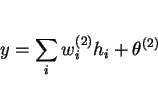
It may be reasonable to assume that the strength of steel microstructures can be factorised into a number of intrinsic components:
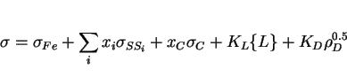 |
(1) |
The individual strengthening contributions are discussed next.
Pure body-centered cubic iron in a fully annealed condition makes an intrinsic (Peierls) contribution ![]() which depends on the temperature (
which depends on the temperature (![]() ) and strain rate (
) and strain rate (![]() ). This dependency on
). This dependency on ![]() and
and ![]() is most pronounced at temperatures less than about -25
is most pronounced at temperatures less than about -25 ![]() C; at
higher temperatures the strength hardly varies, with only a slight decrease consistent with the temperature dependence of the elastic modulus [16; Fig. 1]. The
strength then decreases sharply for temperatures in excess of 600
C; at
higher temperatures the strength hardly varies, with only a slight decrease consistent with the temperature dependence of the elastic modulus [16; Fig. 1]. The
strength then decreases sharply for temperatures in excess of 600 ![]() C; welds in power plant operate at about
600
C; welds in power plant operate at about
600 ![]() C and therefore have to be strengthened with highly stable precipitate phases in order to survive over
a period of about 30 years, the typical design life of such plant. Experimental data for pure iron can be found in [17-19].
C and therefore have to be strengthened with highly stable precipitate phases in order to survive over
a period of about 30 years, the typical design life of such plant. Experimental data for pure iron can be found in [17-19].
![\includegraphics[width=12cm]{fig1.eps}](img42.png) |
Solid solution strengthening due to susbtitutional alloying elements is rather more complicated to treat. The elements have different solubilities in austenite and in ferrite so that they may be distributed non-uniformly in the weld microstructure, which may in any case contain solidification-induced chemical segregation. Notwithstanding the segregation, it turns out that substitutional solutes do not in fact partition during the transformation of austenite to the variety of ferritic phases that are found in welds. This is because martensite, bainite, acicular ferrite and Widmanstätten ferrite grow by a displacive mechanism in which the lattice change is accomplished by a deformation which does not require the diffusion of iron or substitutional solutes [10,20]. The deformation is evident in the invariant-plane strain shape change (with a large shear strain) associated with the growth of each of these phases; the shape deformation also causes a lot of strain which determines the plate shape of all of these transformation products [13]. Allotriomorphic and idiomorphic ferrite, on the other hand, grow by a reconstructive transformation mechanism in which all atoms diffuse to accomplish the lattice change without much strain. Under equilibrium conditions, allotriomorphic ferrite should have a different substitutional solute concentration when compared to the alloy as a whole. However, at the large cooling rates typical of welding, even allotriomorphic ferrite seems to grow by a reconstructive mechanism in which the interface moves at a rate which traps substitutional solutes whether or not they wish to partition. This is called paraequilibrium [21,22,23].
In conclusion, it may reasonably be assumed that the ratio of substitutional-solute to iron atoms in ferritic phases is not different from that calculated from the composition of the steel as a
whole. Solid solution strengthening contributions can therefore be estimated directly from the steel composition (assuming that carbide, nitrides and other phases do not soak up alloying elements).
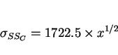
The strengthening contribution ![]() can be estimated as a function of temperature and strain rate from
published data, Fig. 2 [24,25].
can be estimated as a function of temperature and strain rate from
published data, Fig. 2 [24,25].
![\includegraphics[width=12cm]{fig2.eps}](img43.png) |
Fig. 4 shows some interesting typical data [24,25,26]: that whereas the strength of pure iron increases as the temperature is reduced, strengthening due to substitutional solutes often goes through a maximum as a function of temperature, Fig. 3. Indeed, there is some solution softening at low temperatures because the presence of a foreign atom locally assists a dislocation to overcome the exceptionally large Peierls barrier of body-centered cubic iron, at low temperatures. Fig. 3 shows that the solid solution strengthening due to substitutional solutes may reasonably be assumed to vary linearly with concentration.
![\includegraphics[width=12cm]{fig3.eps}](img44.png) |
![\includegraphics[width=12cm]{Table1.eps}](img45.png) |
It is emphasised here that the data presented in Fig. 4 are ``pure", in the sense that they are derived from very careful experiments in which the individual contributions can be measured independently. There exist a vast range of published equations in which the strength is expressed as a (usually linear) function of the weld chemistry [see for example, Table 5.2 of reference 27]. These equations are derived by fitting empirically to experimental data and consequently include much more than just solid solution strengthening components.
Use of the pure data also has the advantage that the solid solution strengthening contribution can be separated from other solute effects. For example, it has been demonstrated [10] that the influence of molybdenum in multirun steel weld deposits is far greater than expected from its solid solution strengthening; there appear to be secondary-hardening effects which are prominent at concentrations greater than about 0.5 wt.%, even when precipitation cannot be observed using conventional transmission electron microscopy.
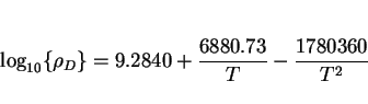
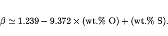
Steels are being designed with ever decreasing interstitial contents. At the same time, processing technology allows accelerated cooling without excessive distortion or microstructural gradients. Lean steels with lower `carbon equivalents' can therefore be manufactured, making fabrication relatively easy. Alloys such as these give uniform microstructures in spite of solidification-induced chemical segregation. Segregated microstructures are more susceptible to stress-corrosion and hydrogen-induced cracking. Consequently, new methods are necessary in order to calculate the microstructure and hence the mechanical properties of the heat-affected zone, the solubility of carbon in ferrite being one of the important factors.
Although the solubility of carbon in ferrite is small and often assumed to be about 0.02 wt.%, it actually changes sharply with temperature and alloy composition (Fig. 5a). The solubility illustrated is when ferrite is in equilibrium with austenite; it will be different (much smaller) when ferrite is in equilibrium with cementite or with any other carbide. The retrograde shape of the phase boundary illustrated in Fig. 5a is a consequence of the detailed thermodynamics of solution of carbon in ferrite [e.g., reference 28] It means that the solubility of ferrite which is in equilibrium with austenite achieves a maximum as a function of temperature; note that the maximum solubility is not at the eutectoid temperature.
The carbon present in ferrite has a major influence on austenite formation in very low carbon steels, and hence on the subsequent development of heat-affected zone microstructures. The effect
illustrated in Fig. 5b [29] is mostly thermodynamic in origin; kinetic factors are less important because both the diffusion coefficient and the driving force
increase with temperature during austenite formation. The temperature at which austenite starts to form during heating is called the ![]() temperature; that at which austenite formation is completed is the
temperature; that at which austenite formation is completed is the ![]() temperature. The slope
of the
temperature. The slope
of the ![]() line (Fig. 5b), and the interval
line (Fig. 5b), and the interval ![]() can be explained directly by reference to the equilibrium Fe-C phase diagram, i.e., by the slope of the
can be explained directly by reference to the equilibrium Fe-C phase diagram, i.e., by the slope of the ![]() phase boundary. An important observation from Fig. 5b
is that very small changes in the carbon concentration of ultra-low carbon steels can have a large effect on microstructural development.
phase boundary. An important observation from Fig. 5b
is that very small changes in the carbon concentration of ultra-low carbon steels can have a large effect on microstructural development.
![\includegraphics[width=12cm]{fig4.eps}](img48.png) |
Martensite can have carbon concentrations which are well in excess of the average concentration in the alloy, because transformation at temperatures above the martensite-start temperature (![]() ) changes the chemical composition of the residual austenite. The total carbon concentration in the alloy (
) changes the chemical composition of the residual austenite. The total carbon concentration in the alloy (![]() ) is the sum of the concentrations in the austenite (
) is the sum of the concentrations in the austenite (![]() ) and ferrite (
) and ferrite (![]() ):
):
 |
(2) |
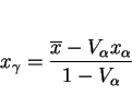 |
(3) |
 |
(4) |
When martensite, bainite, acicular ferrite or Widmanstätten ferrite forms at high temperatures, the shape change due to shear transformation causes plastic deformation, and hence the
accumulation of dislocations in both the parent and product phases [13,20,32]. The extent of the plasticity depends on the yield strength of the parent austenite, and hence on the temperature. The
dislocation density (![]() ) of both martensite and bainite can therefore be represented empirically as a function of
temperature alone (Fig. 6), for the temperature range 570-920 K [33]:
) of both martensite and bainite can therefore be represented empirically as a function of
temperature alone (Fig. 6), for the temperature range 570-920 K [33]:
 |
(5) |
| (6) |
The empirical equation should not be used outside of the stated temperature range. However, it is sometimes necessary to calculate the dislocation density for transformation temperatures which are
less than 570 K. It cannot be assumed that the dislocation density will continue to increase indefinitely as the transformation temperature decreases [34]. Instead it should stabilise at some
limiting value, since any reduction in dislocation density caused by dynamic recovery effects must become negligible at low temperatures. To a good approximation, ![]() for
for ![]() K is given by the value at 570 K.
K is given by the value at 570 K.
![\includegraphics[width=12cm]{fig5.eps}](img67.png) |
Grain boundaries are formidable obstacles to the passage of slip so it is not surprising that they cause strengthening. Stress leads to the generation and flow of dislocations within individual grains. Macroscopic yielding is said to occur when the deformation propagates across adjacent grains. This happens when concentrated stress due to the of a pile up of dislocations at a grain boundary stimulates dislocation sources in adjacent grains. The greater the number of dislocations involved in the original pile-up, the larger is the stress concentration. The number of dilocations that can participate in a pile-up increases with the size of the grain. Thus, the yield strength decreases as the grain size increases.
This is the basis of the classical Hall-Petch relation, in which the increase in strength, ![]() , caused by the
introduction of a grain structure is given by:
, caused by the
introduction of a grain structure is given by:
 |
(7) |
The Hall-Petch relation applies to coarse grained microstructures, since it relies on the existence of sufficient space on a slip plane to build a pile-up or dislocations. Martensite, bainite,
acicular ferrite and Widmanstätten ferrite grow in the form of very fine plates or laths. The mean free path through these plates is only about twice the thickness of the plate; plate thickness
is typically sub-micrometre. Dislocation pile-ups cannot therefore form and the Hall-Petch relation ceases to apply. Instead, yielding involves the spread of dilocations which are present in the
plate boundaries, between pinning points until the resulting loop hits the perimeter of the plate. When the energetics of this process are considered [36,37], the grain size strengthening
becomes:
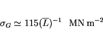 |
(8) |
Great care must be taken in measuring the lineal intercept ![]() , which is measured at random. The
temptation with plate-like structures is to measure the apparent width, i.e., with the test lines lying normal to the plate boundary. Accuracy and randomness are important because of the
sensitivity to strength to small values of
, which is measured at random. The
temptation with plate-like structures is to measure the apparent width, i.e., with the test lines lying normal to the plate boundary. Accuracy and randomness are important because of the
sensitivity to strength to small values of ![]() .
.
We have already seen that the growth of ferrite prior to martensitic transformation can enrich the residual austenite with carbon. The carbon concentration of the martensite that forms
subsequently can be estimated using mass balance (equation 3). The martensite-start temperature (![]() ) of the
residual austenite can be written:
) of the
residual austenite can be written:
 |
(9) |
The Bain strain is a homogeneous pure deformation which can change the face-centered cubic crystal structure of austenite into the body-centered cubic (or tetragonal) structure of martensite. This pure deformation can be combined with a rigid body rotation to give a net lattice deformation which leaves a single line unrotated and undistorted (i.e., an invariant-line strain). In a situation where the transformation is constrained, such a low degree of fit between the parent and product lattices would lead to a great deal of strain as the product phase grows.
However, by adding a further inhomogeneous lattice-invariant deformation (slip or twinning), the combination of deformations appears macroscopically to be an invariant-plane strain [38-40]. Whether the lattice-invariant deformation is slip or twinning is probably determined by kinetic factors such as the mobility of the martensite-austenite interface [41]. As a rough rule, twinned martensite tends to occur when the martensite-start temperature is relatively low.
Weld microstructures often contain small regions of austenite which are enriched with carbon and which subsequently transform to high-carbon martensite during cooling to ambient temperature. These
are the so-called microphases. Transformation twins on ![]() are often found in this high-carbon martensite. This twinned martensite is frequently
suggested to be responsible for bad mechanical properties. It can, however, easily be demonstrated that the twins themselves do not greatly hinder the passage of dislocations [31,40] and so are
unlikely to cause any problems with toughness (Fig. 7). Dislocations can readily traverse the coherent
are often found in this high-carbon martensite. This twinned martensite is frequently
suggested to be responsible for bad mechanical properties. It can, however, easily be demonstrated that the twins themselves do not greatly hinder the passage of dislocations [31,40] and so are
unlikely to cause any problems with toughness (Fig. 7). Dislocations can readily traverse the coherent ![]() twin boundaries body-centered cubic or body-centered tetragonal lattices. It was at one time
believed that the twins were responsible for the high strength of ferrous martensites, because the numerous twin boundaries should hinder slip. This is incorrect because twinned martensites which do
not contain carbon are not particularly strong. It is now generally accepted that the strength of virgin ferrous martensite is largely due to interstitial solid solution hardening by carbon atoms, or
in the case of lightly autotempered martensites due to carbon atom clustering or fine precipitation. Consistent with this, it is found that Fe-30Ni wt.% twinned martensites are not hard.
twin boundaries body-centered cubic or body-centered tetragonal lattices. It was at one time
believed that the twins were responsible for the high strength of ferrous martensites, because the numerous twin boundaries should hinder slip. This is incorrect because twinned martensites which do
not contain carbon are not particularly strong. It is now generally accepted that the strength of virgin ferrous martensite is largely due to interstitial solid solution hardening by carbon atoms, or
in the case of lightly autotempered martensites due to carbon atom clustering or fine precipitation. Consistent with this, it is found that Fe-30Ni wt.% twinned martensites are not hard.
In conclusion, any detrimental effect of the twinned martensite present in the microphases is unlikely to be due to the twins per se, but rather the very high carbon concentration which makes the untempered martensite brittle.
Although glide across coherent twin boundaries in martensite should be unhindered, the boundaries will cause a small amount of hardening. Corresponding slip systems in the matrix and twin will in
general be differently stressed because they are not necessarily parallel [31,42]. Work is also needed to create the steps in the interfaces (Fig. ![]() ). It is emphasized, however, that these should be very minor contributions to the strength of martensite in the microphases found
in weld deposits.
). It is emphasized, however, that these should be very minor contributions to the strength of martensite in the microphases found
in weld deposits.
![\includegraphics[width=12cm]{fig6.eps}](img82.png) |
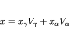
The normal way to calculate the strength of a multiphase alloy is to use a rule of mixtures, i.e., to estimate a mean value from the weighted average of each component:
 |
(10) |
The constraint effect can be explained as follows. It is well established in fracture mechanics that the yield strength is increased by plastic constraint. This is why a weak brazing alloy can be used to bond much stronger samples, as long as the thickness of the braze material is small enough to be constrained throughout by the surrounding stronger matrix. Indeed, the strength of the joint increases as the thickness of the braze layer decreases (Fig. 8).
Dispersions of bainite plates grow in austenite which subsequently transforms to much stronger martensite. This is similar to the brazing analogy. The deformation of the bainitic ferrite can therefore be expected to be constrained by the harder martensite. This can be modelled using experimental data available from brazed joints in high strength steels. As already discussed, the brazing alloys used in making the joints were non-ferrous materials which are ordinarily rather weak. The data, in a normalised form, are summarised in Fig. 8. The vertical axis is the joint strength normalised with respect to that of the unconstrained braze material; the horizontal axis is the braze thickness normalised relative to a thickness value where the restraint effect vanishes.
![\includegraphics[width=12cm]{fig7.eps}](img84.png) |
To analyse the properties of a mixed microstructure of martensite and bainite, it can be assumed that the normalised braze thickness is equivalent to the volume fraction of bainite. Using this
assumption, and the form of the normalised strength versus normalised thickness plot (Fig. 8), the strength of constrained bainite may be represented by the
equation:
![\begin{displaymath}\sigma_b \simeq \sigma_{b0} [0.65 \exp\{-3.3 V_b\} + 0.98] ~~~~ \leq \sigma_M \end{displaymath}](img85.png) |
(11) |
When the volume fraction ![]() of bainite is small, its strength nearly matches that of martensite (Fig. 9), always remaining above that of bainite on its own. The strength of martensite continues to increase with the fraction of bainite, as the carbon concentration of the
residual austenite from which it grows, increases.
of bainite is small, its strength nearly matches that of martensite (Fig. 9), always remaining above that of bainite on its own. The strength of martensite continues to increase with the fraction of bainite, as the carbon concentration of the
residual austenite from which it grows, increases.
![\includegraphics[width=12cm]{fig8.eps}](img90.png) |
Fig. 10 shows a comparison between experimental and calculated data for the strength of the mixed microstructure. Line (a) on Fig. 10 shows that a rule-of-mixtures cannot account properly for the variations observed. The agreement between calculation and experiment improves (curve b) as allowance is made for the change in the strength of martensite as carbon partitions into the austenite, due to the formation of bainite. The consistency between experiment and theory becomes excellent as constraint effects are also included in the calculations (curve c).
![\includegraphics[width=12cm]{fig9.eps}](img91.png) |
Constraint effects are of important in determining the mechanical behaviour of weld microstructures in many respects. Hrivnak [47] has indicated that hard-phase islands present in the heat-affected zone microstructures are most detrimental when they are severely constrained by the surrounding microstructure. Since the constraint is expected to be larger when the island is relatively small, it is these small islands which act as local brittle zones. This is discussed in detail in the section on local brittle zones.
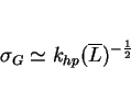
An example calculation of the different factors which contribute to the strength of acicular ferrite is presented in Fig. 10a. The most important contribution other than the intrinsic strength of featureless iron, is the small effective `grain size' of acicular ferrite. As discussed earlier, the mean free slip distance in a plate of acicular ferrite is determined more than anything else by its thickness. It is necessary to consider therefore, the factors which determine the thickness and aspect ratio (i.e., thickness to length ratio) of acicular ferrite plates.
Acicular ferrite is a displacive transformation [10]. The shape deformation associated with a displacive transformation in steel can be described as an invariant-plane strain with a relatively large shear component. Christian [48] demonstrated that when the shape strain is elastically accommodated, the strain energy scales with the plate aspect ratio. This is why all of the displacive transformation products in steel, e.g., Widmanstätten ferrite, bainite, acicular ferrite and martensite, occur in the form of thin plates.
The need to minimise strain energy demands a thin plate, but this also leads to a minimisation of the volume of transformation per plate. Therefore, a plate will tend to adopt the largest aspect ratio consistent with the available free energy change driving the transformation. In ideal circumstances, where the transformation interface remains glissile throughout, and where there is no friction opposing the motion of the interface, thermoelastic equilibrium occurs [32,49,50,51]. The aspect ratio of the plate adjusts so that the strain energy is equal to the driving force, as illustrated in Fig. 10b. The driving force is increased by cooling the austenite, which should lead to plates of increased thickness. Alternatively, it can be decreased by the addition of austenite stabilising elements such as carbon or manganese.
There are good experimental observations [52,53] which have been interpreted recently [54] to support the idea that an increase in the acicular ferrite plate thickness continues until the chemical driving force is exhausted by the accumulation of strain energy. The isolated plates of acicular ferrite which nucleate from point inclusion sites are free to increase in thickness even when their increase in length is restricted by other platelets growing from other inclusions. It is found experimentally that the aspect ratio of acicular ferrite decreases as the transformation temperature is raised, or as the manganese or carbon concentration is increased [52,53].
The idea of thermoelastic equilibrium can therefore be applied to acicular ferrite even though acicular ferrite is probably not entirely elastically accommodated in the matrix. There is thus an easy method for calculating the changes in the acicular ferrite grain size using thermodynamics, an important result given the large grain size strengthening contribution illustrated in Fig. 10a.
|
(a)
![\includegraphics[width=12cm]{fig10a.eps}](img92.png) (b) ![\includegraphics[width=12cm]{fig10b.eps}](img93.png) |
Dislocations also make a significant contribution, but the extent of dislocation strengthening will, unlike the lath size effect, decrease as the transformation temperature increases. Notice that the substitutional solutes make only small contributions to the strength of ferrite. This may be surprising at first sight, since many regression equations describing the strength of welds have much larger coefficients for these solutes. However, those equations do not refer to the solid solution strengthening alone, but to all the effects including for example, any changes in the microstructure caused by alloying. Carbon is not included in Fig. 11 a since its solubility in the ferrite is negligible.
It has been demonstrated that some reasonable assumptions can be made to simplify the calculation of the strength of multirun weld deposits [55]. A volume fraction ![]() is defined to include both the primary microstructure [10], and the reheated regions which are fully austenitised, on the grounds that
these regions are mechanically similar to the as-deposited regions. The remainder
is defined to include both the primary microstructure [10], and the reheated regions which are fully austenitised, on the grounds that
these regions are mechanically similar to the as-deposited regions. The remainder ![]() , includes all the
regions which have been tempered or partially austenitised, and which have lost most of the microstructural component of strengthening.
, includes all the
regions which have been tempered or partially austenitised, and which have lost most of the microstructural component of strengthening. ![]() can be estimated from the alloy chemistry since this in turn influences the extent of the austenite phase field via the
can be estimated from the alloy chemistry since this in turn influences the extent of the austenite phase field via the ![]() temperature [56,57]. It is emphasised that
temperature [56,57]. It is emphasised that ![]() and
and ![]() do not refer to the volume fractions of the primary and secondary microstructures respectively, but are defined in a peculiar way to simplify
the task of estimating the strength of multirun welds. Thus,
do not refer to the volume fractions of the primary and secondary microstructures respectively, but are defined in a peculiar way to simplify
the task of estimating the strength of multirun welds. Thus, ![]() includes the primary microstructure and regions which
are fully austenitised by the deposition of further material, and
includes the primary microstructure and regions which
are fully austenitised by the deposition of further material, and ![]() includes all the other regions which have
essentially lost most of the microstructural component of strength [56,57].
includes all the other regions which have
essentially lost most of the microstructural component of strength [56,57].
The yield strength ![]() of a multirun MMA weld deposit is given by:
of a multirun MMA weld deposit is given by:
 |
(12) |
Fig. 12 shows a series of calculations in which the weld composition is progressively enriched with austenite stabilising elements. Apart from the expected enhancement of strength, increased alloying leads to the following further consequences:
![\includegraphics[width=12cm]{fig11.eps}](img110.png) |
Fig. 13 shows the calculated variations in the strength of submerged-arc all weld metal deposits made with a heat input of about 4 ![]() . There is a systematic variation in the carbon concentration for so-called carbon-manganese
welds containing a variety of other additions. The columnar austenite grain size
. There is a systematic variation in the carbon concentration for so-called carbon-manganese
welds containing a variety of other additions. The columnar austenite grain size ![]() [10] was calculated as a function of the heat input, the carbon, silicon and manganese
concentrations as follows:
[10] was calculated as a function of the heat input, the carbon, silicon and manganese
concentrations as follows:
 |
(13) |
The data in Fig. 13a show that the overall yield and tensile strengths become virtually insensitive to the carbon concentration because of the major effect
of carbon on the austenite grain size. The decrease in hardenability accompanying any reduction in the carbon concentration is virtually compensated by the increase in hardenability due to a larger
austenite grain size. It is believed that the effect of carbon on the austenite grain size comes in via its effect on the ![]() -ferrite to austenite transformation. The columnar austenite grains grow directly from the columnar
-ferrite to austenite transformation. The columnar austenite grains grow directly from the columnar ![]() -ferrite grains. Carbon increases the driving force for
-ferrite grains. Carbon increases the driving force for ![]() reaction, thereby promoting an increase in the nucleation rate of austenite, leading to
a refinement of the grain size.
reaction, thereby promoting an increase in the nucleation rate of austenite, leading to
a refinement of the grain size.
Fig. 13b shows how the strength might have varied with the carbon concentration at a fixed austenite grain size. The intuitively expected trend, that the strength increases with carbon concentration is indeed observed in that case. It is noteworthy that the difference in the strengths of the weakest and strongest regions now increases with the carbon concentration.
![\includegraphics[width=12cm]{fig12.eps}](img117.png) |
The effects of manganese and nickel are illustrated in Fig. 14. The sensitivity to carbon concentration increases as the manganese concentration is increased (Fig. 14a). The addition of nickel is not as effective as that of manganese in changing the strength. A comparison of the change in strength of the 1.5Mn alloy, when a further 1 wt.% of manganese is added to the case where a further 1 wt.% Ni is added shows that the increase is much greater in the former case. This is because manganese has a much larger effect on the hardenability of steel.
![\includegraphics[width=12cm]{fig13.eps}](img118.png) |
There has been a limited amount of progress in the modelling of tensile ductility of the as-deposited microstructure of steel welds [59]. The ductility can to a good approximation be divided into two main components whose magnitudes are assumed to be controlled by different physical processes. These components are the uniform plastic strain, as recorded prior to the onset of macroscopic necking in the tensile specimen, and the nonuniform component which is the remainder of the plastic strain.
By factorising the ductility into these components, it is possible to express the nonuniform component in terms of the inclusion content of the weld deposit, after taking into account variations
in specimen cross-sectional area (![]() ) and gauge length (
) and gauge length (![]() ):
):
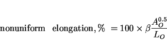 |
(14) |
 |
(15) |
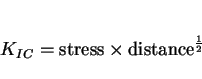
Much of the literature about mechanical toughness tends to focus on micromechanisms, test methodology or procedures for using experimental data in design excercises. By contrast, there is very
little work on the prediction of the ability of complex engineering materials to absorb energy during fracture. This difficulty is illustrated by some basic concepts of fracture mechanics. The
critical value ![]() of the stress intensity which must be exceeded to induce rapid crack propagation is the product
of two terms [60]:
of the stress intensity which must be exceeded to induce rapid crack propagation is the product
of two terms [60]:
 |
(16) |
![\begin{displaymath}\sigma_F \propto\biggl [{{E\gamma_p}\over{\pi(1-\nu^2)c}}\biggr ]^{1\over2} \end{displaymath}](img127.png) |
(17) |
The other parameter in the equation, distance![]() , refers to a distance ahead of the crack tip, within which
the stress is large enough to cause the fracture of brittle crack-initiators. It is well-defined for coarse microstructures but not for many useful microstructures.
, refers to a distance ahead of the crack tip, within which
the stress is large enough to cause the fracture of brittle crack-initiators. It is well-defined for coarse microstructures but not for many useful microstructures.
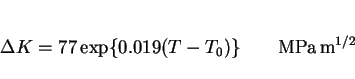
The temperature dependence of the fracture toughness of steels seems to be very well-behaved. Wallin [63,64] has shown that the shape of the toughness versus temperature curve is virtually the
same for all structural steels, making it possible to define a universal dependence as follows:
 |
(18) |
To summarise, there are excellent concepts of fracture mechanics, with established relationships between parameters such as stress and crack-dimensions. These same relationships cannot be used predictively because in each application they rely on experimental data. It is nevertheless true that there is a good qualitative understanding of the factors that control toughness. There are modelling methods which can help convert these qualitative notions into quantitative relationships. These are discussed below in the context of Charpy toughness.
A test used to characterise toughness is the Charpy test, in which a square sectioned, notched bar is fractured under specified conditions [65]. The energy absorbed during fracture is taken as a measure of toughness. The Charpy test is empirical in that the data cannot be used directly in engineering design. It is nevertheless a useful quality control test which is specified widely in international standards, and in the ranking of samples in research and development experiments.
The toughness of a steel depends on many variables, and that of a weld on many more because of the complexity of the welding process. It is not yet possible to predict the Charpy toughness of a weld with any reliability. The usual approach is to correlate the results against chosen variables using linear regression analysis [e.g., reference 66]. These methods are known to be severely limited in their application.
Therefore, the most important mechanical property for welds has not been rationalised quantitatively as a function of the complex array of variables associated with welding. However, it is known from experience, and from the concepts of fracture mechanics, that certain variables are more important than others in their effect on toughness. Given this experience, it should be possible to train an artificial neural network to estimate weld toughness quantitatively as a nonlinear function of these variables, and to see whether the patterns that emerge from the work emulate metallurgical expectations.
In normal regression methods the analysis begins with the prior choice of a relationship (usually linear) between the output and input variables. A neural network is capable of realising a greater variety of nonlinear relationships of considerable complexity. Data are presented to the network in the form of input and output parameters, and the optimum non-linear relationship is found by minimising a penalized likelihood. The network in effect tries out many kinds of relationships in its search for an optimum fit. As in regression analysis, the results then consist of a specification of the function, which in combination with a series of coefficients (called weights), relates the inputs to the outputs. The search for the optimum representation can be computer intensive, but once the process is completed (i.e., the network trained) the estimation of the outputs is very rapid. In spite of its apparent sophistication, the method is as blind as regression analysis, and neural nets can be susceptible to overfitting.
However, much of this danger can in principle be minimised or eliminated by combining the neural network approach with sound statistical and metallurgical theory [67,68,69]
It is possible to choose a set of variables which should, using experience of welding metallurgy, have an influence of the Charpy toughness of weld metal. These variables are listed in Table 2 together with their typical values for high-quality manual metal arc and submerged arc welds.
In general, the toughness decreases as the strength increases. This is because plastic deformation, which is the major energy absorbtion mechanism during fracture, becomes more difficult as the strength increases. Hence, the yield strength is included as a variable. The nature of the welding process itself may have a significant effect on toughness. For example, the submerged arc welding process is quite different from the manual metal arc welding process, leading to the development of different microstructures and variations in impurity content. However, heat input per se is not included since its effect is via the microstructure, which is included in detail in the analysis.
The major solute additions to steels, i.e., C, Mn and Si, have large effects on the transformation behaviour and strength. Impurity elements (P, S, Al, N, O) are included because of their known tendency to embrittle or because of their importance in the formation of nonmetallic inclusions in welds.
All fusion welding processes involve the deposition of a small amount of molten steel within a gap between the components to be joined. When the steel solidifies, it welds the components together. The fusion zone represents both the deposited metal and the parts of the steel component melted during the process, and is a solidification microstructure, often called the primary microstructure [10]. In practice, the gap between the components to be joined has to be filled by a sequence of several weld deposits. These multirun welds have a complicated microstructure. The deposition of each successive layer heat-treats the underlying microstructure. Some of the regions of original primary microstructure are reheated to temperatures high enough to cause the reformation of austenite, which during the cooling part of the thermal cycle transforms into a different microstructure. Other regions may simply be tempered by the deposition of subsequent runs. The microstructure of the reheated regions is called the reheated or secondary microstructure. The fractions of the primary and secondary microstructures are included as input variables (Table 2).
In addition, the details of the primary microstructure are also included in the list of input variables, since the phases involved (allotriomorphic, Widmanstätten and acicular ferrite) are known to have a major influence on the weld properties.
Iron undergoes a ductile-brittle transition as a function of temperature. The flow stress of iron is sensitive to temperature, the strength increasing as the temperature decreases. At some critical temperature, it becomes easier to cleave iron without expending much energy. Below this critical temperature, the iron behaves in a very brittle manner. Hence, the test temperature is included as an important variable.
All of these input variables should to varying degrees influence the Charpy toughness, which is the output variable.
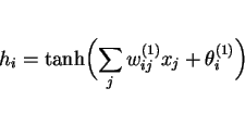
The structure of a typical network used for the analysis is illustrated in Fig. 16.
![\includegraphics[width=12cm]{fig14.eps}](img139.png) |
Linear functions of the inputs ![]() are operated on by a hyperbolic tangent transfer function:
are operated on by a hyperbolic tangent transfer function:
 |
(19) |
 |
(20) |
The complexity of the model is controlled by the number of hidden units (Fig. 16), and the values of the 16 regularisation constants (![]() ), one associated with each input, one for biases and one for all weights connected to the output.
), one associated with each input, one for biases and one for all weights connected to the output.
![\includegraphics[width=12cm]{fig15.eps}](img147.png) |
Fig. 17 shows that the inferred noise level decreases monotonically as the number of hidden units increases. However, the complexity of the model also
increases with the number of hidden units. A high degree of complexity may not be justified, and in an extreme case, the model may in a meaningless way attempt to fit the noise in the experimental
data. MacKay [67,68] has made a detailed study of this problem and has defined a quantity (the evidence) which comments on the probability of a model. In circumstances where two models give
similar results over the known dataset, the more probable model would be predicted to be that which is simpler; this simple model would have a higher value of `evidence'. The evidence framework was
used to control the regularisation constants and ![]() . The number of hidden units was set by examining
performance on test data. A combination of Bayesian and pragmatic statistical techniques were therefore used to control the model complexity. Four hidden units were found to give a reasonable level
of complexity to represent the variations in toughness as a function of the input variables. Larger numbers of hidden units did not give significantly lower values of
. The number of hidden units was set by examining
performance on test data. A combination of Bayesian and pragmatic statistical techniques were therefore used to control the model complexity. Four hidden units were found to give a reasonable level
of complexity to represent the variations in toughness as a function of the input variables. Larger numbers of hidden units did not give significantly lower values of ![]() ; indeed, the test set error goes through a minimum at four hidden units (Fig. 18).
; indeed, the test set error goes through a minimum at four hidden units (Fig. 18).
The optimum parameters for one trained network are presented later in Table 3; this listing would be required in order to reproduce the predictions described, though not the error bars. The levels of agreement for the training and test datasets are illustrated in Fig. 19, which show good prediction in both instances. It should be emphasized that the test data were not included in deriving the weights given in Table 3 (except to choose the solution displayed), so that the good fit is established to work well over the range of data included in the analysis.
We now examine the metallurgical significance of the results [69]. We attempt predictions out of the range of the experimental data used during training, and examine some aspects which cannot be studied experimentally.
Fig. 20 illustrates the significance (![]() ) of each of the input
variables, as perceived by the neural network, in influencing the toughness of the weld. The process clearly has a large intrinsic effect, which complies with experience in that submerged arc welds
are in general of a lower quality than manual metal arc welds. Note that this is a process effect which is independent of all the other variables listed. The yield strength has a large effect and
that is well established [65]. It is also widely believed, as seen in Fig. 20, that ferrite has a large effect on the toughness. Nitrogen has a large effect,
as is well established experimentally [70-75]. Oxygen influences welds in both beneficial and harmful ways, e.g., by helping the nucleation of acicular ferrite or contributing to fracture by
nucleating oxides.
) of each of the input
variables, as perceived by the neural network, in influencing the toughness of the weld. The process clearly has a large intrinsic effect, which complies with experience in that submerged arc welds
are in general of a lower quality than manual metal arc welds. Note that this is a process effect which is independent of all the other variables listed. The yield strength has a large effect and
that is well established [65]. It is also widely believed, as seen in Fig. 20, that ferrite has a large effect on the toughness. Nitrogen has a large effect,
as is well established experimentally [70-75]. Oxygen influences welds in both beneficial and harmful ways, e.g., by helping the nucleation of acicular ferrite or contributing to fracture by
nucleating oxides.
It is surprising at first sight that carbon has such a small effect, but what the results really demonstrate is that the influence of carbon comes in via the strength and microstructure.
Phosphorus and sulphur have only a small effect; the toughness measured was in the as-welded condition whereas many of the classical embrittlement effects manifest themselves in the stress-relieved
condition. It is also possible that the effects of P and S are higher at strength levels larger than encountered here. All of the welding consumables are commercially used so that they are not
expected to be embrittlement prone. Elements such as Mn and Si do not feature greatly presumably because their effect comes in via microstructure. Fig. 20 also
shows a relatively small effect of temperature on toughness, but it should be noted that the temperature range considered is only 80 ![]() C, and that a part of the effect of temperature is to alter the yield strength, which is identified by the model to be one of the important variables.
C, and that a part of the effect of temperature is to alter the yield strength, which is identified by the model to be one of the important variables.
![\includegraphics[width=16cm]{fig18.eps}](img150.png) |
The model can be used to estimate the toughness if all of the inputs listed in Table 2 are available. The amount of work required to accumulate these inputs is not trivial, but the situation can be ameliorated. A physical model [10] based on phase transformation theory can be used to predict the values of all the inputs from a knowledge of just the chemical composition and a choice of welding conditions. This was done particularly to examine the effects of carbon and manganese on weld toughness, given that a lot of work on these lines has already been reported in the literature.
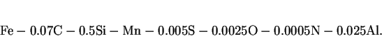
Fig. 21 a shows data generated using the neural network but with all the inputs other than manganese calculated using our weld model [10]. In all cases, the
calculated inputs are for manual metal arc welds with 180 A, 34 V, a welding speed of 0.004 ![]() , interpass temperature 200
, interpass temperature 200 ![]() C, ISO2569 weld geometry. The manganese variations are for a basic composition
C, ISO2569 weld geometry. The manganese variations are for a basic composition
 |
(21) |
Fig. 21b shows similar data for carbon (the only difference being that the Mn concentration is fixed at 1 wt.%.). The explanation is identical to that for the Mn data.
![\includegraphics[width=12cm]{fig19.eps}](img152.png) |
For welds similar to the carbon series, but with the carbon concentration fixed at 0.07 wt.%, the oxygen concentration alone was varied to a range well outside of the training dataset. These
results are presented in Fig. 22 along with the ![]() standard deviation
predicted error bars. It is clear that any attempt to extrapolate beyond the dataset on which the model is based gives predictions which are not terribly useful. The fact that the toughness increases
with oxygen at low concentrations is strange since the acicular ferrite content (and indeed all the other inputs) are kept constant. An increase in the oxygen content alone should lead to a
deterioration in toughness because of the tendency for non-metallic oxide particles to initiate fracture.
standard deviation
predicted error bars. It is clear that any attempt to extrapolate beyond the dataset on which the model is based gives predictions which are not terribly useful. The fact that the toughness increases
with oxygen at low concentrations is strange since the acicular ferrite content (and indeed all the other inputs) are kept constant. An increase in the oxygen content alone should lead to a
deterioration in toughness because of the tendency for non-metallic oxide particles to initiate fracture.
![\includegraphics[width=12cm]{fig20.eps}](img154.png) |
Finally, it is possible using the model to examine effects which cannot easily be produced experimentally. It has frequently been argued that acicular ferrite is a better microstructure than Widmanstätten ferrite, because the former with its less organised arrangement of ferrite plates has a greater capacity to deflect cracks. This was tested for a manual metal arc weld containing 0.07 wt.% carbon but of otherwise identical composition to the carbon series of welds (Fig. 6). The allotriomorphic ferrite fraction was set to zero and all inputs except acicular ferrite and Widmanstätten ferrite were varied in a complementary fashion. The results (Fig. 23) are exciting - they demonstrate that increased acicular ferrite leads to an improvement of cleavage toughness but not of the upper shelf energy - the latter is not expected to change since the strengths of acicular and Widmanstätten ferrite are virtually identical [59].
![\includegraphics[width=12cm]{fig21.eps}](img155.png) |
Table 3 contains the values for the weights obtained after completing the training of the network. These data can be used in combination with Table 2 and equations 19,20 in order to use the network to make predictions of weld metal toughness.
It has been accepted for some time that allotriomorphic ferrite (![]() ) is bad for weld metal toughness because
it offers little resistance to cleavage crack propagation. However, this kind of ferrite grows by a reconstructive mechanism in which all of the atoms diffuse. Thus, grains of
) is bad for weld metal toughness because
it offers little resistance to cleavage crack propagation. However, this kind of ferrite grows by a reconstructive mechanism in which all of the atoms diffuse. Thus, grains of ![]() can grow freely across austenite grain boundaries. Displacive transformations (Widmanstätten ferrite, bainite, acicular
ferrite, martensite) on the other hand, involve the coordinated motion of atoms. Such movements cannot be sustained across grain boundaries. Hence, in a fully transformed microstructure, a vestige of
the austenite grain boundary remains when the transformation is displacive. In the presence of impurities, this can lead to intergranular failure with respect to the prior austenite grain boundaries.
With allotriomorphic ferrite, the original
can grow freely across austenite grain boundaries. Displacive transformations (Widmanstätten ferrite, bainite, acicular
ferrite, martensite) on the other hand, involve the coordinated motion of atoms. Such movements cannot be sustained across grain boundaries. Hence, in a fully transformed microstructure, a vestige of
the austenite grain boundary remains when the transformation is displacive. In the presence of impurities, this can lead to intergranular failure with respect to the prior austenite grain boundaries.
With allotriomorphic ferrite, the original ![]() boundaries are entirely disrupted, removing the site for the
segregation of impurities. This conclusion is supported by observations reported in the literature. Abson [78] examined a large set of weld deposits. Of these, a particular weld which had no
allotriomorphic ferrite content and a particularly high concentration of phosphorus exhibited brittle failure at the prior columnar austenite grain boundaries in the manner illustrated in
Fig. 24.
boundaries are entirely disrupted, removing the site for the
segregation of impurities. This conclusion is supported by observations reported in the literature. Abson [78] examined a large set of weld deposits. Of these, a particular weld which had no
allotriomorphic ferrite content and a particularly high concentration of phosphorus exhibited brittle failure at the prior columnar austenite grain boundaries in the manner illustrated in
Fig. 24.
It is well known that the post-weld heat treatment (600 ![]() C) of titanium and boron containing welds leads to
embrittlement with failure at the columnar austenite grain boundaries [79-81]. Phosphorus has been shown to segregate to these prior austenite boundaries and cause a deterioration in the toughness.
The titanium and boron make the welds sensitive to post-weld heat treatment because they prevent allotriomorphic ferrite, and hence expose the remains of the austenite grain boundaries to impurity
segregation.
C) of titanium and boron containing welds leads to
embrittlement with failure at the columnar austenite grain boundaries [79-81]. Phosphorus has been shown to segregate to these prior austenite boundaries and cause a deterioration in the toughness.
The titanium and boron make the welds sensitive to post-weld heat treatment because they prevent allotriomorphic ferrite, and hence expose the remains of the austenite grain boundaries to impurity
segregation.
Kayali et al. [82] and Lazor and Kerr [83] have reported such intergranular failure, again in welds containing a fully acicular ferrite microstructure. Sneider and Kerr [84] have noted that such fracture appears to be encouraged by excessive alloying. Boron is important in this respect because it can lead to an elimination of austenite grain boundary nucleated phases; recent observations on intergranular fracture at the prior austenite boundaries [85] can be interpreted in this way. This is consistent with our hypothesis, since large concentrations austenite-stabilising elements tend to reduce the allotriomorphic ferrite content.
It must be emphasised that it is not the reduction in allotriomorphic ferrite content per se which worsens the properties; the important factor is the degree of coverage (and hence disruption) of the prior austenite grain surfaces. In addition, the impurity content has to be high enough to cause embrittlement. Classical theory suggests that additions of elements like molybdenum should mitigate the effects of impurity controlled embrittlement, although such ideas need to be tested for the as-deposited microstructure of steel welds. To summarise, it is likely that allotriomorphic ferrite should not entirely be designed out of weld microstructures, especially if the weld metal is likely to contain impurities.
![\includegraphics[width=12cm]{fig22.eps}](img158.png) |
Recent work reinforces the conclusion that some allotriomorphic ferrite should be retained in the weld microstructure in order to improve its high temperature mechanical properties. Ichikawa et al. [86] examined the mechanical properties of large heat input submerged arc welds designed for fire-resistant steels. They demonstrated that the high temperature ductility and the creep rupture life of the welds deteriorated sharply in the absence of allotriomorphic ferrite (Fig. 25). The associated intergranular fracture at the prior austenite grain boundaries, became intragranular when allotriomorphic ferrite was introduced into the microstructure.
![\includegraphics[width=12cm]{fig23.eps}](img159.png) |
Steel can be infiltrated at the prior austenite grain boundaries by liquid zinc. In a study of the heat-affected zone of steel welds, Iezawa et al. [87] demonstrated that their susceptibility to liquid zinc embrittlement depended on the allotriomorphic ferrite content, which in turn varied with the boron concentration (Fig. 26). The absence of allotriomorphs at the prior austenite grain boundaries clearly made them more sensitive to zinc infiltration, proving again that these prior boundaries have a high-energy structure which is susceptible to wetting and impurity segregation.
![\includegraphics[width=12cm]{fig24.eps}](img160.png) |
The rutile based electrode systems currently under development generally lead to phosphorus concentrations of about 0.010-0.015 wt.%, and the popular use of titanium and boron gives a weld deposit without allotriomorphic ferrite. The welds have therefore been found to be extremely susceptible to stress relief embrittlement with fracture along the prior austenite grain boundaries. Possible solutions include:
It was argued above that with displacive transformations (which cannot cross austenite grain boundaries), a ``vestige" of the austenite grain boundary structure is left in the microstructure. The following evidence suggests that these prior austenite grain boundaries are high-energy boundaries:
The misfit present at austenite grain boundaries can evidently be inherited in a fully transformed specimen. This is because the displacive transformation of austenite involves a minimal movement
of atoms. The Bain Strain, which is the pure component of the deformation which converts the austenite lattice into that of ferrite, does not rotate any plane or direction by more than about ![]() [100]. Furthermore, the change in volume during transformation is a few percent. The excellent registry between
the parent and product lattices is illustrated by the electron diffraction pattern of Fig. 27.
[100]. Furthermore, the change in volume during transformation is a few percent. The excellent registry between
the parent and product lattices is illustrated by the electron diffraction pattern of Fig. 27.
Consequently, the detailed arrangement of atoms at an austenite grain boundary is unlikely to be influenced greatly by displacive phase transformation.
There are many investigations which suggest that Widmanstätten ferrite can be detrimental to toughness [101-110]. Recent work involving controlled experiments has, however, established that when the microstructure is changed from one which is predominantly allotriomorphic ferrite, to one containing Widmanstätten ferrite, there is an improvement in both the toughness and strength [111]. This might be expected since large fractions of Widmanstätten ferrite are usually associated with refined microstructures.
It is sometimes claimed that the presence of Widmanstätten ferrite changes the deformation behaviour by inducing continuous yielding during tensile deformation, whereas discontinuous yielding is characteristic of microstructures dominated by allotriomorphic ferrite. However, some careful studies by Bodnar and Hansen [111] show that even microstructures containing Widmanstätten ferrite often show discontinuous yielding behaviour. They suggested that in cases where continuous yielding has been reported, the microstructures contained sufficient quantities of bainite or martensite to mask the deformation behaviour of Widmanstätten ferrite.
An acicular ferrite microstructure is usually assumed to be good for the achievement of a high cleavage toughness. This is because the plates of ferrite point in many different directions, and hence are able to frequently deflect cracks. This should give better toughness when compared with allotriomorphic ferrite, or even Widmanstätten ferrite or bainite, which tends to form in packets of parallel plates (across which cracks can propagate with relative ease). However, good evidence to this latter effect has been lacking. An example is illustrated in Fig. 28, where the fracture assessed impact transition temperature is plotted as a function of the strength and microstructure [112]. It is obvious that the progressive replacement of a coarse allotriomorphic ferrite microstructure with acicular ferrite, even though the strength increases in the process.
As acicular ferrite is then replaced with bainite, the toughness deteriorates, but the cause of this is not straightforward to interpret because the strength increases at the same time (Fig. 28).
![\includegraphics[width=12cm]{fig26.eps}](img164.png) |
Similar observations have recently been reported for both wrought steel and for weld metal [113]. The data presented in Fig. 29 demonstrate again the fact that an acicular ferrite microstructure is desirable even though non-metallic inclusions have to be added in order to provide intragranular nucleation sites.
![\includegraphics[width=8cm]{fig27.eps}](img165.png) |
Knott and co-workers have suggested that once a crack is initiated at an inclusion, it propagates without hindrance by acicular ferrite. Recent work by Ishikawa and Haze [114] has demonstrated that whilst this must be true when the general level of toughness is small, the gradient of stress at any position in the vicinity of a crack decreases as the toughness increases. Hence, the propagation behaviour changes, and cleavage cracks are then arrested in an acicular ferrite microstructure but not in one which is dominated by Widmanstätten ferrite.
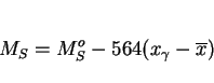
``Microphase" is the term used to describe the small amount of martensite, austenite, degenerate-pearlite which forms after all the other phases (allotriomorphic ferrite, Widmanstätten ferrite, acicular ferrite) have formed. The fraction of the microstructure which is left untransformed after the major phases have formed is very small in most low-alloy low-carbon steels; hence the term microphases. Microphases are also found in the heat-affected zones of welded steels.
The chemical composition of the microphases is for the substitutional solutes, identical to that of the alloy as a whole, but is substantially enriched with respect to the carbon concentration
[115,116; Fig. ![]() ]. The excess carbon is due to partitioning as the major
phases grow. It is interesting (Fig.
]. The excess carbon is due to partitioning as the major
phases grow. It is interesting (Fig. ![]() ) that the degree of carbon
enrichment is found to increase as the cooling rate decreases. This is because as the cooling rate decreases, the volume fraction of ferrite that grows prior to microphase formation is larger. Hence,
by mass balance, the carbon concentration of the residual austenite is expected to be larger.
) that the degree of carbon
enrichment is found to increase as the cooling rate decreases. This is because as the cooling rate decreases, the volume fraction of ferrite that grows prior to microphase formation is larger. Hence,
by mass balance, the carbon concentration of the residual austenite is expected to be larger.
![\includegraphics[width=12cm]{fig29.eps}](img166.png) |
It is generally recognised that microphases occur in two main morphologies, those originating from films of austenite which are trapped between parallel plates of ferrite, and others which are blocky in appearance.
The mechanism by which the microphases influence toughness in low-alloy steels (strength about 800 MPa) have been studied in detail by Chen et al. [117]. The effects vary with the test temperature. The films of hard phases tend to crack readily when loaded along their longest dimensions, often splitting into several segments. The blocks of microphases, on the other hand, tend to remain uncracked. At high temperatures, the cracks in the films initiate voids and hence lead to a reduction in the work of ductile fracture. The ferrite, which is softer and deforms first, has a relatively low strength at high temperatures and cannot induce fracture in the blocky microphases. The latter only come into prominence at low temperatures, where their presence induces stresses in the adjacent ferrite, stresses which peak at some distance ahead of the microphase/ferrite interface. This induces cleavage in the ferrite. Larger blocks are more detrimental in this respect because the peak stress induced in the adjacent ferrite is correspondingly larger.
Fracture mechanics are widely applied in the design of engineering structures, but difficulties arise when repeated tests of the kind used in characterising toughness, on the same material, yield significantly different results. Such scatter in toughness is a common feature of relatively brittle materials such as ceramics, where it is a key factor limiting their wider application even when the average toughness may be acceptable. Steel users have become increasingly aware in recent years that scatter in toughness data can also be of concern in wrought and welded steels. Apart from the difficulties in adopting values for design purposes, the tests necessary for the characterisation of toughness as a material property are rather expensive, the number of experiments needed to establish confidence being larger for less unreliable materials.
A major factor responsible for variations in toughness in welds is likely to be the inclusion population which consists mainly of large oxides originating from the slags used to control the weld pool stability and composition. The inclusions are neither uniform in size, nor are they uniformly distributed in the weld. There is also mounting evidence that variations in microstructure can also be an important factor in influencing scatter in toughness data [118-122]. Neville [123] noted that microstructural inhomogeneities such as hard pearlite islands, can lead to a significant variations in measured fracture toughness values during repeat tests on specimens of the same material.
The two quantities that need to be defined in order to assess variations in mechanical properties are the degree of scatter, and the heterogeneity of microstructure. The definitions have to be of a kind amenable to alloy design techniques, while at the same time being physically meaningful.
Consider the scatter commonly observed in impact toughness data. The three most frequently used ways of rationalising variations in results from the toughness testing of weld metals are to take an average of the Charpy readings obtained at a given temperature, measure the standard deviation [124], or plot the lowest Charpy readings obtained in order to focus attention on the lower ends of the scatter bands [125].
An alternative to this was suggested by Smith [126] who proposed a scatter factor ![]() to quantify any spread
obtained in Charpy values, where
to quantify any spread
obtained in Charpy values, where
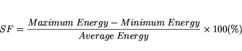 |
(22) |
None of the methods discussed above are completely suitable for alloy design purposes, where the aim is to minimise scatter over the whole of the impact transition curve (the plot of impact energy versus test temperature). An idealised impact energy-temperature curve should be sigmoidal in shape, and the scatter of experimental data can in principle be measured as a root-mean-square deviation about a such a curve, obtained by best-fitting to the experimental data. This gives a representation of scatter in which one value of scatter is defined for each complete impact transition curve. It has the advantage that the value represents the entire dataset used in generating the transition curve.
Since it is believed that the scatter in Charpy data is amongst other factors, dependent on the nonuniformity of weld microstructure, the degree of inhomogeneity needs to be quantified. This can
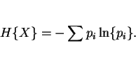
be done by calculating the entropy ![]() of a given microstructure [127,128].
of a given microstructure [127,128].
If ![]() is a random variable assuming the value
is a random variable assuming the value ![]() with probability
with probability ![]() ,
, ![]() , the entropy of
, the entropy of ![]() , as a logarithmic measure of the mean probability, is computed according to
, as a logarithmic measure of the mean probability, is computed according to
 |
(23) |
The primary microstructure of most common welds can be taken as having three principal constituents: acicular, allotriomorphic and Widmanstätten ferrite. It is important to emphasise that
although ![]() and
and ![]() have
similar strengths, the weld metal microstructure cannot be treated as a two-phase microstructure (with
have
similar strengths, the weld metal microstructure cannot be treated as a two-phase microstructure (with ![]() and
and
![]() grouped together), since the toughness values of the two phases are quite different. Therefore, the
entropy of a given weld metal microstructure
grouped together), since the toughness values of the two phases are quite different. Therefore, the
entropy of a given weld metal microstructure
![\begin{displaymath}H = - [V_\alpha \ln \{V_\alpha\} + V_a \ln \{V_a\} + V_w \ln \{V_w\}] \end{displaymath}](img178.png) |
(24) |
The entropy of the distribution quantifies the heterogeneity of the microstructure. ![]() will vary from zero for an
homogeneous material to
will vary from zero for an
homogeneous material to ![]() (i.e. 1.099) for a weld with equal volume fractions of the three phases. By
multiplying by
(i.e. 1.099) for a weld with equal volume fractions of the three phases. By
multiplying by ![]() , the heterogeneity of the three phase microstructure of a weld may be defined on a scale
from zero to unity, i.e.
, the heterogeneity of the three phase microstructure of a weld may be defined on a scale
from zero to unity, i.e.
 |
(25) |
![\begin{displaymath}Het_2 = - [V_p\ln \{V_p\} + V_s\ln \{V_s\}] \times {{1} \over {\ln \{2\}}} \end{displaymath}](img184.png) |
(26) |
It is evident from (Fig. 31a) that there is a strong relationship between the scale parameter, and microstructural heterogeneity for low-alloy steel all-weld metals. Consequently, a significant part of the observed scatter in weld metal Charpy results is attributable to the inhomogeneity of the microstructure, with larger scatter being associated empirically with more heterogeneous microstructures. This result can be compared with the common feature of fracture toughness experiments where the positioning of the fatigue crack is found to be an important factor in CTOD testing of weldments.
![\includegraphics[width=12cm]{fig30.eps}](img187.png) |
Copper has two primary effects, firstly to retard the transformation of austenite (since it is an austenite stabilising element), and secondly to strengthen ferrite via the precipitation of ![]() -Cu.
-Cu.
In manual metal arc welds, copper increases the strength, but at concentrations in excess of about 0.7 wt.% to a deterioration in toughness in both the as-welded and stress-relieved states [129]. There may be a simple explanation for this, in that an increase in strength should indeed lead to a deterioration of toughness, since the comparisons are never at constant strength.
Kluken et al. [85] showed that in submerged arc welds, the yield strength is less sensitive to copper additions than the ultimate tensile strength, perhaps because the copper precipitates cause a greater rate of work hardening. On the other hand, Es-Souni et al. [129] found the rate of change, as a function of the copper concentration, to be identical for both the yield and tensile strengths, in manual metal arc welds.
The austenite stabilising effect of copper seems to cause either an increase in the microphase content, or changes the nature of the microphases from cementite and ferrite to mixtures of retained austenite and high-carbon martensite [129,130]. The presence of copper has not been found to influence either the distribution or the nature of the usual non-metallic inclusions found in steel weld deposits [129].
Hydrogen is a key parameter controlling the mechanical properties of welded assemblies. There has been a fascinating development on the methods available for the directional removal of hydrogen following a welding operation. It is, however, necessary to describe first some background theory to set the idea into context.
In all our discussions of thermodynamics, we have dealt with measurable properties of materials, formulated on the concept of equilibrium. There are, however, many properties of nonequilibrium systems (thermal conductivity, diffusion, viscosity etc.) which are similar to thermodynamic properties, such as temperature, density or entropy, in that their definitions are not based on the structure of matter. Nonequilibrium thermodynamics, or the thermodynamics of irreversible processes deals with the relations between such properties [131,132].
Classical thermodynamics only applies to systems which are in equilibrium. A reversible process is one which can be reversed by an infinitesimal change in the external conditions [133]. If we consider the motion of a piston in a cylinder containing a compressible fluid, the reversible motion of the piston in the cylinder would lead to a pressure-volume relation illustrated by the light curve of Fig. 32. Any friction to the motion of the piston would make the process irreversible since an infinitesimal application of force would not move that piston. Energy (given by the area within the bold loop of Fig. 32) would therefore be dissipated during the cyclic frictional motion of the piston, a key feature of irreversible processes.
![\includegraphics[width=12cm]{fig31.eps}](img189.png) |
More generally then, reversibility means that one can pass from one state to another without appreciable deviation from equilibrium. Most real process are, therefore, not reversible. For
irreversible processes the equations of classical thermodynamics become inequalities. For example, at the equilibrium melting temperature, the free energies ![]() but below the melting temperature,
but below the melting temperature, ![]() . Such inequalities are much less useful and provide information only about the
direction of likely change.
. Such inequalities are much less useful and provide information only about the
direction of likely change.
There is however, some rough (kinetic) theory which can allow us to relate the magnitude of the inequality to the rate of change. Such theory is controversial in an interesting sense, and lacks generality [131]. The assumptions involved must be verified experimentally. On the other hand, once backed by experiment, quantitative deductions and predictions become possible.
At equilibrium there is no change in entropy or free energy. For any irreversible process, there is energy dissipated. In the above example, it is the heat that is created by friction that leads
to dissipation of energy and the creation of entropy. The energy dissipation rate can be expressed as the product of the temperature and rate of entropy production (![]() ). The dissipation is always found to be of the form:
). The dissipation is always found to be of the form:
 |
(27) |
A major result of kinetic theory for nonequilibrium processes is that forces and their conjugate fluxes are linearly related whenever the above equation applies.
The force may be a chemical driving force (![]() ), an electromotive force (e.m.f.) (
), an electromotive force (e.m.f.) (![]() ), a thermal gradient
), a thermal gradient ![]() etc. The corresponding fluxes might be interface velocity (
etc. The corresponding fluxes might be interface velocity (![]() ), electrical current (
), electrical current (![]() ) and heat
diffusion (
) and heat
diffusion (![]() ) respectively.
) respectively.
 |
(28) |
 |
(29) |
 |
(30) |
Many irreversible processes acting together can easily be handled, because the total energy dissipation rate is simply
 |
(31) |
For more than one irreversible process, it is found experimentally that each flow ![]() is related not only to its
conjugate force
is related not only to its
conjugate force ![]() , but is also linearly related to all other forces present. Thus,
, but is also linearly related to all other forces present. Thus,
 |
(32) |
Solute diffusion can therefore be expressed as a function of both the chemical potential gradient and the e.m.f. as follows:
 |
(33) |
There is an example in processing where hydrogen is used to induce the disintegration of a material. In the hydrogen decrepitation process, sintered solids are charged with hydrogen, causing them to crumble, thus producing the desired powder for further processing [135,136]. The process is used for making sintered magnets. It would be interesting to exploit such metallurgical phenomena to help in the catastrophic or gradual destruction of large steel structures.
Obsolete oil rigs are massive steel structures which have to be decommissioned safely. Some rigs are disposed by using explosives to sever them into two parts, both of which are sunk into the ocean, taking care to leave about 55 m of clear water above the sunken components for free navigation. It would be an advantage if these large sunken segments could deteriorate quickly into much smaller segements on the ocean floor. One possibility is to charge localised regions of the rigs with hydrogen, so that hydrogen cracking then leads to further underwater disintegration of the large segments over a short period of time after the sinking. Bead-on-plate welds could be deposited at critical nodes, the welding being carried out using electrodes which have a high carbon concentration and a number of water-containing minerals. This would lead to a hard deposit with a great deal of hydrogen, thus not only charging the underlying rig-steel with hydrogen but also providing sharp cracks in the weld which can then propagate into the substrate. It may be the case that self-stress in the rig would then be sufficient to permit the large scale propagation of cold-cracks.
Microstructural models are in many cases sufficiently advanced to give accurate predictions for welds. It is now necessary to focus attention on the relationship between microstructure and mechanical properties, so that data useful as design parameters can easily be generated.
It has been demonstrated here that both simple and complex mechanical properties can be modelled with considerable success if appropriate modelling techniques are used. Parameters such as strength have a firm foundation in metallurgy and can indeed be estimated using known metallurgical principles. Others such as toughness are less amenable to fundamental analysis but can nevertheless be modelled using pattern recognition methods. A great deal of work remains to be done before comprehensive models for all the desired properties can be constructed; a priority list of the properties which need analysis is presented in Table 4.
I am grateful to Colin Humphreys for his continuing support of my research and also sincerely acknowledge the long term support of welding research by Dr. Lars-Erik Svennson of ESAB AB (Sweden). The Engineering and Physical Sciences Research Council provided some financial support over the years.
8mm
.
1, (Alberry, P. J. and Jones, W. K. C.) 1979 CEGB report R/M/R282, Marchwood Engineering Laboratories, Marchwood, Southampton, U. K.
2, (Alberry, P. J. and Jones, W. K. C.) 1982 Metals Technology, 9, 419-427.
3, (Alberry, P. J., Brunnstrom, R. R. L. and Jones, K. E.) 1983 Metals Technology, 10, 28-38.
4, (Ashby, M. F. and Easterling, K. E.) 1982 Acta Metallurgica, 30, 1969-1978.
5, (Ion, C., Easterling, K. E. and Ashby, M. F.) 1984 Acta Metallurgica, 32, 1949-1962.
6, (Goldak, J., Chakravarti, A. and Bibby, M.) 1984 Metallurgical Transactions B, 15B, 299-305.
7, (Goldak, J., Bibby, M., Moore, J., House, R. and Patel, B.) 1986 Metallurgical Transactions B, 17B, 587-600.
8, (Bhadeshia, H. K. D. H.) 1989 Recent Trends in Welding Science and Technology, eds. S. A. David and J. M. Vitek, ASM International, Ohio, U. S. A., 189-198.
9, (Bhadeshia, H. K. D. H.) 1990 Metallurgy, Welding and Qualification of Microalloyed (HSLA) Steel Weldments, eds. J. T. Hickey, D. G. Howden and M. D. Randall, American Welding Society, Florida, U.S.A., 34-69
10, (Bhadeshia, H. K. D. H. and Svensson, L.-E.) 1993 Mathematical Modelling of Weld Phenomena, eds. H. Cerjak and K. E. Easterling, Institute of Materials, London, 109-182.
11, (Olson, D. L., Liu, S. and Edwards, G. R.) 1993 Mathematical Modelling of Weld Phenomena, eds. H. Cerjak and K. E. Easterling, Institute of Materials, London, 89-108.
12, (Grong, ![]() .) 1995 Metallurgical Modelling of Welding, Institute of Materials, London, 1-600.
.) 1995 Metallurgical Modelling of Welding, Institute of Materials, London, 1-600.
13, (Bhadeshia, H. K. D. H.) 1995 Mathematical Modelling of Weld Phenomena 2, eds. H. Cerjak and H. K. D. H. Bhadeshia, Institute of Materials, London, 71-118.
14, (Kranszberg, M. and Smith, C. S.) 1979 Materials Science and Engineering, 37,30.
15, (Radaj, D.) 1995 Mathematical Modelling of Weld Phenomena 2, eds. H. Cerjak and H. K. D. H. Bhadeshia, Institute of Materials, London, 245-264.
16, (Leslie, W. C.) 1982 Physical Metallurgy of Steels, McGraw-Hill Kogakusha, Tokyo, Japan.
17, (Conrad, H. and Fredrick, S.) 1962 Acta Metallurgica, 10,1013-1020.
18, (Altshuler, T. L. and Christian, J. W.) 1967 Proceedings of the Royal Society, 261A,253-287.
19, (Kimura, H., Matsui, H., Takaki, S., Kimura, A. and Oguri, K.) 1981 Mechanical Properties of BCC Metals, ed. M. Meshii, The Metallurgical Society of AIME, Warrendale, Pennsylvania, 125-133.
20, (Bhadeshia, H. K. D. H.) 1992 Bainite in Steels, Institute of Materials, London, 1-458.
21, (Hultgren, A.) 1951 Jernkontorets Ann., 135, 403.
22, (Hillert, M.) 1952 Jernkontorets Ann., 136, 25-37.
23, (Bhadeshia, H. K. D. H.) 1985 Progress in Materials Science, 29, 321-386.
24, (Leslie, W. C.) 1972 Metallurgical Transactions, 3,5-26.
25, (Takeuchi, S.) 1969 Journal of the Physical Society of Japan, 27,929-940.
26, (Honeycombe, R. W. K. and Bhadeshia, H. K. D. H.) 1995 Steels, Microstructure and Properties, 2nd edition, Edward Arnold, London.
27, (Svensson, L.-E.) 1994 Control of Microstructure and Properties in Steel Arc Welds, CRC Press, London.
28, (Bhadeshia, H. K. D. H.) 1982 Metal Science, 16, 167-169.
29, (Abiko, K.) June 1993 Scientific American, Japanese edition, 20-29.
30, (Maki, T.) 1994 Physical Metallurgy of IF Steels, Iron and Steel Institute of Japan, Tokyo, 183-197.
31, (Christian, J. W.) 1971 Strengthening Methods in Crystals, eds. A. Kelly and R. Nicholson, Elsevier, North-Holland, 261-329.
32, (Christian, J. W.) 1979 Proceedings of an International Conference on Martensitic Transformations, ICOMAT '79, M.I.T. press, Cambridge, Massachusetts, U.S.A., 220-234.
33, (Takahashi, M. and Bhadeshia, H. K. D. H.) 1990 Materials Science and Technology, 6 592-603.
34, (Young, C. H. and Bhadeshia, H. K. D. H.) 1994 Materials Science and Technology, 10,209-214.
35, (Yang J. R. and Bhadeshia, H. K. D. H.) 1990 The Dislocation Density of Acicular Ferrite in Steel Welds, Welding Journal Research Supplement, 69,305s-307s.
36, (Langford, G. and Cohen, M.) 1969 Trans. ASM, 62,623.
37, (Langford, G. and Cohen, M.) 1970 Metallurgical Transactions, 1,1478-1480.
38, (Wechsler, W. S., Lieberman, D. S. and Reed, T. A.) 1953 Trans. AIMME, 197,1503-1515.
39, (Bowles, J. S. and MacKenzie, J. K.) 1954 Acta Metallurgica, 2,129-234.
40, (Bhadeshia, H. K. D. H.) 1987 Worked Examples in The Geometry of Crystals, Institute of Metals, London.
41, (Olson, G. B. and Cohen, M.) 1981 Solid![]() Solid Phase Transformations, eds. H. I. Aaronson
et al., TMS-AIME, Warrendale, Pennsylvania, USA, 1209.
Solid Phase Transformations, eds. H. I. Aaronson
et al., TMS-AIME, Warrendale, Pennsylvania, USA, 1209.
42, (Kelly, P. M. and Pollard, G.) 1969 Acta Metallurgica, 17,1005.
43, (Tomita, Y. and Okabayashi, K.) 1983 Metallurgical Transactions A, 14A,485-492.
44, (Tomita, Y. and Okabayashi, K.) 1983 Metallurgical Transactions A, 14A,2387-2393.
45, (Tomita, Y. and Okabayashi, K.) 1985 Metallurgical Transactions A, 16A,73-82.
46, (Tomita, Y. and Okabayashi, K.) 1985 Metallurgical Transactions A, 16A,83-91.
47, (I. Hrivnak) 1996 Mathematical Modelling of Weld Phenomena 3, eds. H. Cerjak, B. Buchmayer and H. K. D. H. Bhadeshia, Institute of Materials, London, in press.
48, (Christian, J. W.) 1958 Acta Metallurgica, 6,377-379.
49, (Kurdjumov, G. V. and Khandros, L. G.) 1949 Dokl. Akad. Nauk SSSR, 66,221.
50, (Olson, G. B. and Cohen, M.) 1977 Scripta Metallurgica, 11,345-347.
51, (Salzbrenner, R. J. and Cohen, M.) 1979 Acta Metallurgica, 27,739-748.
52, (Court, S. and Pollard, J.) 1987 Welding Metallurgy of Structural Steels, ed. J. Y. Koo, TMS-AIME, Pennsylvania, 335-349.
53, (Zhang, Zhu Yau) 1994 Ph.D. Thesis, Southampton University.
54, (Chang, L. C. and Bhadeshia, H. K. D. H.) 1995 Materials Science and Technology, in press.
55, (Sugden, A. A. B. and Bhadeshia, H. K. D. H.) 1988 Metallurgical Transactions A, 19A,1597-1602.
56, (Svensson, L.-E. and Bhadeshia, H. K. D. H.) 1988 Improved Weldment Control using Computer Technology, Vienna, Austria, Pergamon Press, Oxford, 71-78.
57, (Svensson, L.-E., Gretoft, B., Sugden, A. A. B. and Bhadeshia, H. K. D. H.) 1988 Computer Technology in Welding II, Welding Institute, Abingdon, UK, paper 24.
58, (Jones, B. L. and Johnson, D. L.) 1983 Steels for Line-Pipe and Pipeline Fittings, Metals Society, London, 14.
59, (Sugden, A. A. B. and Bhadeshia, H. K. D. H.) 1989 J. Materials Science, 25, 613-618.
60, (Knott, J. F.) 1995 Micromechanisms of Fracture and Their Structural Significance, Second Griffith Conference, Institute of Materials, London, 3-14.
61, (McMahon Jr., C. J. and Cohen, M.) 1965 Acta Metallurgica, 13,591.
62, (D. A. Curry and J. F. Knott) 1978 Metal Science, 12,511.
63, (Wallin, K.) 1993 International Journal of Pressure Vessels and Piping, 55,61-79.
64, (Wallin, K.) 1995 Micromechanisms of Fracture and Their Structural Significance, Second Griffith Conference, Institute of Materials, London, 131-140.
65, (Knott, J. F.) 1973 Fundamentals of Fracture Mechanics, Butterworths, London, 8.
66, (Akselsen, O. M. and Grong, ![]() .) 1992 Materials Science and Engineering A, A159, 187-192.
.) 1992 Materials Science and Engineering A, A159, 187-192.
67, (MacKay, D. J. C.) 1992a Neural Computation, 4, 415-447.
68, (MacKay, D. J. C.) 1992b Neural Computation, 4, 448-472.
69, (Bhadeshia, H. K. D. H., Svensson, L.-E. and Mackay, D. J. C.) 1995 Materials Science and Technology, in press.
70, (Lau, T. W., Sadowsky, M. M., North, T. H. and Weatherly, G. C.) 1987 Welding Metallurgy of Structural Steels, ed. J. Y. Koo, T.M.S.-A.I.M.E., Warrendale, Pennsylvania, U.S.A., 349-365.
71, (Lau, T. W., Sadowsky, M. M., North, T. H. and Weatherly, G. C.) 1988 Materials Science and Technology, 4, 52-61.
72, (Oldland, R. B.) December 1985 Australian Welding Research, 31-43.
73, (Ahlblom, B., Bergstrom, U., Hannerz, N. E. and Werlefors, I.) 1986 WI conference on Residuals and Impurities in Steels Welding Insititute, Abington, Cambridge, U. K., paper 49
74, (Grong, ![]() , Kluken, A. O. and Bjornbakk, B.) 1988 Joining and Materials, 1, 164-169.
, Kluken, A. O. and Bjornbakk, B.) 1988 Joining and Materials, 1, 164-169.
75, (Liou, H. Y., Liao, C. M. and Wang, S. C.) 1992 China Steel Technical Report No. 6, 30-37.
76, (Evans, G. M.) 1980 American Welding Journal, 59, 67s-75s.
77, (Svensson, L.-E. and Gretoft, B.) 1990 American Welding Journal, 69, 454s-461s.
78, (Abson, D. J.) 1988 Welding Institute Research Report 376/1988, Cambridge, UK.
79, (Still, J. R. and Rogerson, J. H.) 1978 Metal Construction, 10, 339-342.
80, (Still, J. R. and Rogerson, J. H.) 1980 Metal Construction, 12, 120-123.
81, (Kluken, A. O. and Grong, ![]() ) 1992 Temper embrittlement in steel weld metals containing titanium and
boron International Trends in Welding Science and Technology eds. S. A. David and J. M. Vitek, ASM International, Metals Park, Ohio, U. S. A., 569-574.
) 1992 Temper embrittlement in steel weld metals containing titanium and
boron International Trends in Welding Science and Technology eds. S. A. David and J. M. Vitek, ASM International, Metals Park, Ohio, U. S. A., 569-574.
82, (Kayali, E. S., Pacey, A. J. and Kerr, H. W.) 1984 Canadian Metallurgical Quarterly, 23,227-236.
83, (Lazor, R. B. and Kerr, H. W.) 1980 Pipeline and Energy Plant Piping: Design and Technology, Pergamon Press, Toronto, Canada, 141-149.
84, (Sneider, G. and Kerr, H. W.) 1984 Canadian Metallurgical Quarterly, 23, 315-325.
85, (Kluken, A. O., Siewert, T. A. and Smith, R.) 1994 Effects of copper, nickel and boron on mechanical properties of low-alloy steel weld metals deposited at high heat input American Welding Journal, 73, 193s-199s.
86, (Ichikawa, K., Horii, Y., Motomatsu, R., Yamaguchi, M. and Yurioka, N.) 1994 Quarterly Journal of the Japan Welding Society, in press.
87, (Iezawa, T., Inoue, T., Hirano, O., Okazawa, T. and Koseki, T.) 1993 Tetsu to Hagane, 79,96-102.
88, (Briant, C. L. and Banerji, S. K.) 1978 International Metals Reviews, 232, 164-199.
89, (Schulz, B. J. and McMahon Jr., C. J.) 1972 Temper Embrittlement of Alloy Steels, STP 499, American Society for Testing and Metals, 104.
90, (McMahon Jr., C. J., Cianelli, A. K., Feng, H. C. and Ucisik, A. H.) 1977 Metallurgical Transactions A, 8A, 1059.
91, (Yu, J. and McMahon Jr., C. J.) 1980 Metallurgical Transactions A, 11A, 291.
92, (McMahon Jr., C. J. and Qu Zhe) 1983 Metallurgical Transactions A, 14A, 1101.
93, (Krauss, G. and McMahon Jr., C. J.) 1992 Martensite, eds. G. B. Olson and W. S. Owen, ASM International, Materials Park, Ohio, U.S.A., 295-322.
94, (Steven, W. and Balajiva, K.) 1959 J. Iron and Steel Institute, 193, 141.
95, (Yu-Qing, W. and McMahon Jr., C. J.) 1986 Supplement to Trans. Japan Inst. Metals, 27, 579.
96, (McMahon Jr., C. J.) 1987 Innovations in ultrahigh-strength steel technology, eds. G. B. Olson, M. Azrin and B. S. Wright, Sagamore Army Research Conference, Northwestern University, U.S.A., 597-618.
97, (Hyam, E. D. and Nutting, J.) 1956 Journal of the Iron and Steel Institute, 184,148-165.
98, (Baker, R. G. and J. Nutting) 1959 Journal of the Iron and Steel Institute, 192,257-268.
99, (Vander Vroot, G. F.) 1984 Metallography, Principles and Practice, McGraw-Hill Book Company, London, 219-223.
100, (Crosky, A., McDougall, P. G. and Bowles, J. S.) 1980 Acta Metallurgica, 28,1495-1504.
101, (Owen, W. S., Whitmore, D. H., Cohen, M. and Averbach, B. L.) 1957 Welding Journal Research Supplement, November, 503s-511s.
102, (Gulyaev, A. P. and Guzovskaya, M. A.) 1977 Met. Sci. Heat Treat., 19, 1020-1024.
103, (Koval'chuk, G. Z., Geichenko, V. N., Yarmosh, V. N. and Podobedova, L. V.) 1979 Met. Sci. Heat Treat., 21, 114-117.
104, (Chilton, J. M. and Roberts, M. J.) 1979 Vanadium in High Strength Steels, Vanitec, London, 11-21.
105, (Chilton, J. M. and Roberts, M. J.) 1980 Metallurgical Transactions A, 11A, 1711-1721.
106, (Otterberg, R., Sandrom, R. and Sandberg, A.) 1980 Metals Technology, 7, 397-408.
107, (Stenbacka, N.) 1980 Scandanavian Journal of Metallurgy, 9, 225-236.
108, (Morrison, W. B. and Preston, R. R.) 1984 Proc. Int. Symp. on Niobium, edited by H. Stuart, TMS-AIME, Warrendale, PA, 939-966.
109, (Glover, G., Oldland, R. B. and Voight, G.) 1984 High-Strength, Low-Alloy Steels, eds. D. P. Dunne and T. Chandra, South Coast Printers, New South Wales, Australia, 271-275.
110, (Huang, Z. and Yao, M.) 1989 Materials Science and Engineering A, A119, 211-217.
111, (Bodnar, R. L. and Hansen, S. S.) 1994 Metallurgical and Materials Transactions A, 25A, 763-773.
112, (Horii, Y. and Ohkita, S.) 1992 Welding International, 6, 761-765.
113, (Harrison, P. L. and Hart, P. H. M.) 1995 Micromechanisms of Fracture and Their Structural Significance, Second Griffith Conference, Institute of Materials, London, 57-68.
114, (Ishikawa, T. and Haze, T.) 1994 Materials Science and Engineering A, A176, 385-391.
115, (Komizo, Y. and Fukada, Y.) 1989 CTOD properties and MA constituent in the HAZ of C-Mn Microalloyed Steel, The Sumitomo Search, No. 40, 31-40.
116, (Matsuda, F., Li, Z., Bernasovsky, P., Ishihara, K. and Okada, H.) 1990 An Investigation of the Behaviour of M-A constituent in Simulated HAZ of HSLA steels, IIW Document IX-B-1591-90.
117, (Chen, J. H., Kikuta, Y., Araki, T., Yoneda, M. and Matsuda, Y.) 1984 Acta Metallurgica, 32, 1779-1788.
118, (Tweed, J. H. and Knott, J. F.) 1983 Metal Science, 17, 45-54.
119, (Tweed, J. H. and Knott, J. F.) 1987 Acta Metallurgica, 35, 1401-1414.
120, (Bowen, P., Druce, S. G. and Knott, J. F.) 1986 Acta Metallurgica, 34, 1121-1131.
121, (Neville, D. and Knott, J. F.) 1986 J. Mechanics and Physics of Solids, 34, 243-291.
122, (Hagiwara, Y. and Knott, J. F.) 1980 Advances in Fracture Research, ed. D. Francois, Pergamon Press, Oxford, U. K. 707.
123, (Neville, D.) 1985 Ph.D. Thesis, University of Cambridge, U. K.
124, (Drury, B. G.) 1984 Welding and Metal Fabrication, 53, 250-252.
125, (Taylor, D. S.) 1982 Welding and Metal Fabrication, 50, 452-460.
126, (Smith, E.) 1983 Welding and Metal Fabrication, 51, 210-204.
127, (Lange, F. H.) 1967 Correlation Techniques, Iliffe Books Ltd., London, U. K. 76-77.
128, (Karlin, S. and Taylor, H. M.) 1975 A First Course in Stochastic Processes, Academic Press, New York, U. S. A., 495-502.
129, (Es-Souni, M., Beaven, P. A. and Evans, G. M.) 1990 Microstructure and mechanical properties of Cu-bearing MMA C-Mn weld metal Oerlikon Schweibmitteilungen, No. 123, 15-31.
130, (Alekseev, A. A., Shevchenko, G. A., Pokhodnya, I. K. and Yurlov, B. V.) 1991 Effect of copper on structure and properties of multilayer C-Mn-Ni weld metal IIW Document II-A-845-91, 1-7.
131, (Christian, J. W.) 1975 Theory of Transformations in Metals and Alloys, 2nd ed., Part I, Pergamon Press, Oxford.
132, (Miller, D. G.) 1960 Chemical Reviews, 60,15-37.
133, (Pippard, A. B.) 1981 The Elements of Classical Thermodynamics, Cambridge University Press, Cambridge, U. K., 22.
134, (Mishra, B., Olson, D. L. and David, S. A.) 1995 Journal of Materials Engineering and Performance, 3,612-618.
135, (Harris, I. R.) 1985 Journal of the Less-Common Metals, 106,L1.
136, (Harris, I. R.) 1987 Journal of the Less-Common Metals, 131,245.
![\includegraphics[width=12cm]{Table2.eps}](img138.png)
![\includegraphics[width=12cm]{fig16.eps}](img148.png)
![\includegraphics[width=12cm]{fig17.eps}](img149.png)
![\includegraphics[width=14cm]{Table3.eps}](img156.png)
![\includegraphics[width=12cm]{fig25.eps}](img163.png)
![\includegraphics[width=12cm]{fig32.eps}](img212.png)
![\includegraphics[width=14cm]{Table4.eps}](img213.png)