
A model has been created to allow the quantitative estimation of the fatigue crack growth rate in steels as a function of mechanical properties, test-specimen characteristics, stress-intensity range and test–frequency. With this design, the remarkable result is that the method which is based on steels, can be used without modification, and without any prior fatigue test, to estimate the crack growth rates in nickel, titanium and aluminium alloys. It appears therefore that a large proportion of the differences in the fatigue crack growth rate of metallic alloys can be explained in terms of the macroscopic tensile properties of the material rather than the details of the microstructure and chemical composition.
Materials and Design, 31 (2010) 2134-2139.
R. C. Dimitriu and H. K. D. H. Bhadeshia
A model has been created to allow the quantitative estimation of the fatigue crack growth rate in steels as a function of mechanical properties, test-specimen characteristics, stress-intensity range and test-frequency. With this design, the remarkable result is that the method which is based on steels, can be used without modification, and without any prior fatigue test, to estimate the crack growth rates in nickel, titanium and aluminium alloys. It appears therefore that a large proportion of the differences in the fatigue crack growth rate of metallic alloys can be explained in terms of the macroscopic tensile properties of the material rather than the details of the microstructure and chemical composition.
Keywords: Fatigue Crack Growth, Neural Network, Steel, Superalloys, Titanium Alloys, Aluminium Alloys
It is understood that fatigue crack growth is a consequence of the accumulation of damage by deformation in the plastic zone at the crack tip. At low loads the deformation is governed by the cyclic variation in the stress-intensity range ![]() . The crack extension per cycle
. The crack extension per cycle ![]() becomes measurable at a threshold
becomes measurable at a threshold
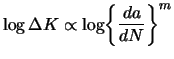
![]() , followed by the slower extension rate in the Paris Law regime [4,2,1,3] described by the proportionality
, followed by the slower extension rate in the Paris Law regime [4,2,1,3] described by the proportionality
 |
(1) |
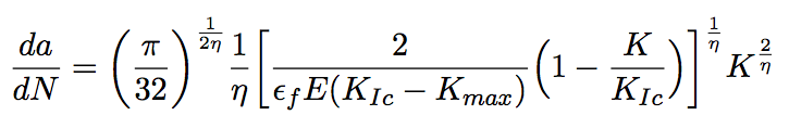
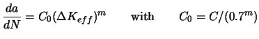
Elber modified the relation with an effective stress intensity range
![]() to allow for variable amplitude loading, arguing that cracks grow only when their tips are open [7]:
to allow for variable amplitude loading, arguing that cracks grow only when their tips are open [7]:
 |
(2) |
![$\displaystyle \frac{da}{dN} = \bigg( \frac{\pi}{32} \bigg)^{\frac{1}{2\eta}} \f... ... ) } \Big(1 - \frac{K}{K_{Ic}} \Big) \bigg]^{\frac{1}{\eta}} K^{\frac{2}{\eta}}$](./fatigue/img14.png) |
(3) |
The aim here was to exploit published fatigue crack growth data to create a model based on physical variables which are readily measured in a tensile test, rather than rely on inputs which depend on fatigue testing, and further, to include variables which account for test-specimen parameters. The model uses neural network analysis; although there are physically based models available in the literature, for example, [10], they require fitting parameters; a neural network is the most general way of achieving fitting without making prior assumptions about the relationship to which the data are fitted [11]. There have been other attempts to use neural networks for this purpose [12] but they do not adequately treat the uncertainties of modelling so it is not possible to properly assess the predictions made. The original intention here was to study steels, but as will be seen later, the model was, without modification, found to generalise to other alloy systems.
A versatile method for treating empirical data is the neural network in a Bayesian framework. The theory behind practical Bayesian networks has been described in [14,13] and the background information theory is available in a seminal textbook on the subject [15]. In addition, this method been reviewed thoroughly [11], as have been its applications [16]. Indeed, there have been diverse applications which lead to useful and verifiable predictions in the context of low-cycle fatigue [17], the estimation of bainite plate thickness [18], the calculation of ferrite number in stainless steels [19], the estimation of tensile strength [20,27], impact strength [26,21], the effect of processing parameters on marageing steels [22], the modelling of strain induced martensitic transformation [23], and the reduction in steel varieties [28], to name but a few. There has even been an assessment of procedures needed to design networks which are well-assessed in their performance [24]. Given this plethora of literature, only specific points of relevance are introduced here.
With neural networks, the input data ![]() are multiplied by weights, but the sum of all these products forms the argument of a flexible mathematical function (known as the transfer function), here a hyperbolic tangent. The output
are multiplied by weights, but the sum of all these products forms the argument of a flexible mathematical function (known as the transfer function), here a hyperbolic tangent. The output ![]() is therefore a non-linear function of
is therefore a non-linear function of ![]() . The exact shape of the hyperbolic tangent can be varied by altering the weights. Further degrees of non-linearity can be introduced by combining several of these hyperbolic tangents, so that the network is able to model highly non-linear relationships. The nature of the transfer functions and the weights define a reproducible mathematical function which represents the empirical data.
. The exact shape of the hyperbolic tangent can be varied by altering the weights. Further degrees of non-linearity can be introduced by combining several of these hyperbolic tangents, so that the network is able to model highly non-linear relationships. The nature of the transfer functions and the weights define a reproducible mathematical function which represents the empirical data.
The network just described is essentially a non-linear regression method which, because of its flexibility, is able to capture complicated data, whilst at the same time avoiding overfitting. There are a number of interesting outputs other than the coefficients which help recognise the significance of each input. First, there is the noise in the output, associated with the fact the input set is unlikely to be comprehensive - i.e., a different result is obtained from identical experiments. Secondly, there is the uncertainty of modelling because many mathematical functions may be able to adequately represent known data but which behave differently when extrapolated. A knowledge of this uncertainty helps make the method less risky in extrapolation. This uncertainty can be expected to be large in regions of the input domain where data are sparse or exceptionally noisy.
Published [25] fatigue crack growth data for tests done in ordinary air, at room temperature, were digitised, covering steels with chemical compositions in the range presented in Table 1. Traces element concentrations (Ti, Al, V, S, P) together with the details of heat treatment can be found in the original compilation [25]. The properties of a steel depend on the composition and heat treatment, but fatigue crack propagation should depend to a large extent on macroscopic mechanical properties. It was deliberately decided to focus on easily measured properties obtained from a tensile test, rather than use inputs such as the threshold stress intensity which would defeat the purpose of modelling since a fatigue test would be required before a prediction could be made. The dimensions of the test specimens and the test conditions are also important in this respect and were included in the analysis. The advantage of this approach also is that a large quantity of data are available with each of the input variables listed in Table 1. Data for both axial mode I and an in-plane bending mode II were incorporated; mode III data were not available.
The plots in Fig. 1 illustrate the distribution of data, but clearly cannot represent multidimensional dependencies. However, the neural network method used here is based on a Bayesian framework [15,13] so that the predictions are associated with a modelling uncertainty whose magnitude depends on the position in the input domain where a calculation is done. . As pointed out previously, the details of the neural network and Bayesian framework used have been fully described elsewhere so only the essential points are included in this paper.
The data were randomly and equally divided into the training and testing sets, and normalised [11]. One hundred networks were trained, with hidden units ranging from one to twenty and five seeds in each case. This is in order to select a committee of models which gives the best generalisation on unseen data [29,14,13,11]. The performance of the optimum committee accompanies by
![]() modelling uncertainties is illustrated in Fig. 2. Of the total of 12807 data, only 158 can be classified as mild outliers which are more than 3
modelling uncertainties is illustrated in Fig. 2. Of the total of 12807 data, only 158 can be classified as mild outliers which are more than 3![]() from the measured values. The noise in the output of the committee model was found to be
from the measured values. The noise in the output of the committee model was found to be
![]() , which is a constant additional error to the modelling uncertainties plotted in subsequent graphs. The network perceived significances, which indicate the ability of an input to explain the variation in the output (akin a partial correlation coefficient) are shown in Fig. 3. The elongation, ultimate tensile strength and proof stress are significant in influencing
, which is a constant additional error to the modelling uncertainties plotted in subsequent graphs. The network perceived significances, which indicate the ability of an input to explain the variation in the output (akin a partial correlation coefficient) are shown in Fig. 3. The elongation, ultimate tensile strength and proof stress are significant in influencing ![]() but it is natural that the stress intensity range
but it is natural that the stress intensity range ![]() should have the greatest effect. Although it is expected in a valid test that specimen size should not influence
should have the greatest effect. Although it is expected in a valid test that specimen size should not influence ![]() [30], it is likely that true plane strain conditions do not exist in all the cases studied, and hence a specimen size effect is perceived in Fig. 3. Such behaviour has been reported previously, with the crack growth rate increasing as plane-strain conditions are approached [31].
[30], it is likely that true plane strain conditions do not exist in all the cases studied, and hence a specimen size effect is perceived in Fig. 3. Such behaviour has been reported previously, with the crack growth rate increasing as plane-strain conditions are approached [31].
One way of assessing a model is by making predictions, in this case on a bearing steel of relevance in our other research. The steel of interest is variously known as SUJ2, AISI 52100 and En31 in different countries and has the approximate composition 1C, 0.3-1.1Mn, 1.2-1.4Cr, 0.2-0.4Si wt%. The inputs required were obtained from [32]: 5% elongation, 2030 MPa 0.2% proof stress, 2240 MPa tensile strength, loading mode 2, specimen length 80 mm, specimen thickness 2 mm, pre-crack size 3 mm, frequency 2 Hz and stress ratio 0.
Fig. 4 shows the outcome, with the model not only capturing the trend in the variation of ![]() versus
versus ![]() over several orders of magnitude, and both for the threshold and Paris regions of the curve, but giving also a reasonable absolute prediction accuracy.
over several orders of magnitude, and both for the threshold and Paris regions of the curve, but giving also a reasonable absolute prediction accuracy.
Although all of the data used to create the model were from experiments on steels [25], the inputs include only mechanical and test parameters. It was imagined that the model should therefore apply without modification to other alloys.
Calculations for three nickel-base superalloys Udimet 700, Inconel 718 and Waspaloy; their detailed compositions can be found in [36,37,34,35,33]. Fig. 5 compares the model and the experimental data using the inputs listed in Table 2. The calculations are represented with the uncertainty range and the reported measurements [36,37,34,35,33] as points. The results are fascinating since the model correctly estimates the Paris slopes, although it marginally overestimates the fatigue behaviour (we have checked that this overestimation is not explained by modulus variations between the different materials). A similar level of agreement was found for titanium Ti-6Al-4V, 7075 aluminium alloy were made and compared against published measurements [38,39], Fig. 6. The model nicely captured the slope for both the titanium and aluminium alloys, and it again slightly overestimates the fatigue crack growth rates.
In order to further test the model a colleague from industry supplied input data (last two columns, Table 2) without revealing the alloy type for the purpose of making blind predictions, for which the crack growth rates would be revealed after the calculations are made. Fig. 7 shows calculations, and the subsequent experimental data on the same Ti6Al4V alloy with two different heat treatments. The agreement obtained is good.
The computer program associated with this work can be downloaded freely from:
RCD would like to thank the European Commission, Marie Curie Early Stage Research Training Programme.
.
| Variable | Figure number | |||||||||
| 5a | 5b | 5c | 5d | 5e | 5f | 6a | 6b | 7a | 7b | |
| Elongation / % | 5 | 15 | 20 | 20 | 27 | 33 | 14 | 8 | 20 | 14 |
| 0.2% Proof stress / MPa | 1020 | 1172 | 1113 | 1113 | 1076 | 921 | 930 | 524 | 1172 | 940 |
| Tensile strength / MPa | 1520 | 1404 | 1373 | 1373 | 1441 | 1351 | 970 | 464 | 1440 | 998 |
| Specimen length / mm | 72.5 | 63.5 | 50.8 | 31.8 | 62.5 | 5 | 155 | 155 | 7 | 7 |
| Specimen thickness / mm | 12.5 | 25.4 | 12.7 | 8.89 | 25 | 3 | 40 | 40 | 7 | 7 |
| Pre-crack length / mm | 12.5 | 18.3 | 6.4 | 5.3 | 17.5 | 0.4 | 9 | 9 | 0.5 | 0.5 |
| Stress ratio | 0.1 | 0.1 | 0.05 | 0.05 | 0.5 | 0.5 | -1 | 0.5 | 0.1 | 0.5 |
| Frequency / Hz | 40 | 20 | 0.667 | 0.667 | 20 | 100 | 20 | 20 | 0.25 | 100 |
![\includegraphics[width=0.95\textwidth]{sig22.eps}](./fatigue/img40.png)
|
![\includegraphics[width=10cm]{pred111.eps}](./fatigue/img41.png)
|
|
[a]
![\includegraphics[width=0.40\textwidth]{100.eps}](./fatigue/img42.png) [b] [b]![\includegraphics[width=0.40\textwidth]{101.eps}](./fatigue/img43.png) [c] [c]![\includegraphics[width=0.40\textwidth]{102.eps}](./fatigue/img44.png) [d] [d]![\includegraphics[width=0.42\textwidth]{103.eps}](./fatigue/img45.png) [e] [e]![\includegraphics[width=0.40\textwidth]{105.eps}](./fatigue/img46.png) [f] [f]![\includegraphics[width=0.40\textwidth]{106.eps}](./fatigue/img47.png)
|
|
[a]
![\includegraphics[width=0.42\textwidth]{TiAlV.eps}](./fatigue/img48.png) [b] [b]![\includegraphics[width=0.42\textwidth]{7075.eps}](./fatigue/img49.png)
|
|
|
|
|
|
| Pipeline texture | Mathematical Models | Bake hardening | Nuclear | 301L stainless |
| Residual stress | TRIP | 301L stainless | Hot-strength | Intervention |
| δ-TRIP | Metallography | Bearings | Topology | Tiny bainite |
| PT Group Home | Materials Algorithms |
![\includegraphics[width=0.32\textwidth]{elv.eps}](./fatigue/img30.png)
![\includegraphics[width=0.32\textwidth]{tens.eps}](./fatigue/img31.png)
![\includegraphics[width=0.32\textwidth]{profstre.eps}](./fatigue/img32.png)
![\includegraphics[width=0.32\textwidth]{speclengt.eps}](./fatigue/img33.png)
![\includegraphics[width=0.32\textwidth]{specwidt.eps}](./fatigue/img34.png)
![\includegraphics[width=0.32\textwidth]{specpre.eps}](./fatigue/img35.png)
![\includegraphics[width=0.32\textwidth]{stresrati.eps}](./fatigue/img36.png)
![\includegraphics[width=0.32\textwidth]{freque1.eps}](./fatigue/img37.png)
![\includegraphics[width=0.32\textwidth]{logdkda.eps}](./fatigue/img38.png)
![\includegraphics[width=0.75\textwidth]{pvmcomch2.eps}](./fatigue/img39.png)
![\includegraphics[width=0.42\textwidth]{bt11.eps}](./fatigue/img50.png) [b]
[b]![\includegraphics[width=0.42\textwidth]{bt22.eps}](./fatigue/img51.png)