
The purpose here is to help identify the microstructures in steel using simple techniques based on the atomic mechanisms by which phases grow from austenite. Apart from their aesthetic beauty, microstructures become meaningful when examined in the context of their metallurgical theory. You can freely download the complete book Theory of Transformations in Steels.
The symbols used to represent each phase are as follows:
| Phase | Symbol | Phase | Symbol |
|---|---|---|---|
| Austenite | γ | Allotriomorphic ferrite | α |
| Idiomorphic ferrite | αI | Pearlite | P |
| Widmanstätten ferrite | αw | Upper bainite | αb |
| Lower bainite | αlb | Acicular ferrite | αa |
| Martensite | α′ | Cementite | θ |
We shall interpret microstructures in the context of the iron-carbon equilibrium phase diagram, even though steels inevitably contain other solutes, whether by design or as impurities.
 Figure 1: Crystal structures of austenite, ferrite and cementite, and the Fe-C equilibrium phase diagram. Only the front-facing face-centring atoms are illustrated for austenite for the sake of clarity.
Austenite has a cubic-close packed crystal structure (fcc). Ferrite (α) is body-centred cubic (bcc) and cementite (θ) is orthorhombic (Fe3C). Equilibrium phase fractions can also be estimated from a knowledge of the carbon concentration of the steel and an application of the lever rule.
Understanding atomic mechanisms is vital as atom movement determines morphology and composition.
 Figure 2: The displacive and reconstructive mechanisms.
In the displacive mechanism, the change occurs without disrupting atomic order (homogeneous deformation). In the reconstructive mechanism, bonds are broken and atoms rearranged structure-by-structure via diffusion.
 Figure 3: Classification of phases according to atomic mechanisms.
The kinetics are illustrated using a time-temperature-transformation (TTT) diagram.
 Figure 4: Time-temperature-transformation diagram.
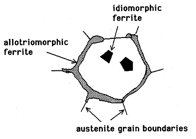 Figure 5: Grain boundary allotriomorph of ferrite, and intragranular idiomorph.
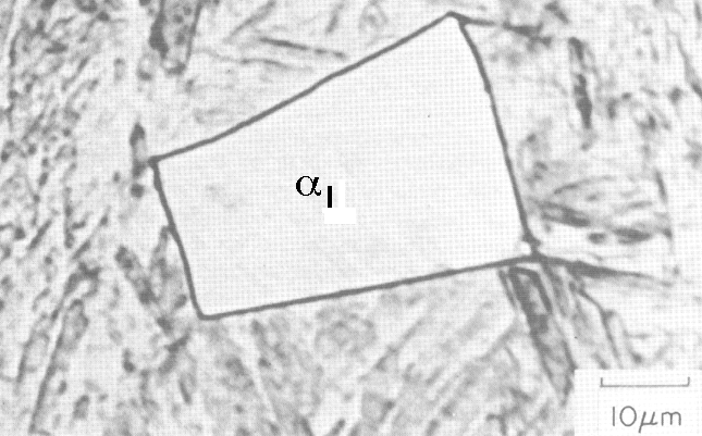 Figure 6: An idiomorph of ferrite in a sample which is partially transformed into α and then quenched.
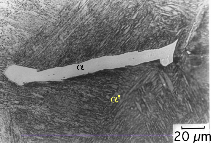 Figure 7: An allotriomorph of ferrite growing rapidly along the austenite grain boundary.
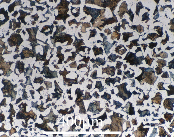 Figure 8: Allotriomorphic ferrite in a Fe-0.4C steel; the dark-etching microstructure is fine pearlite.
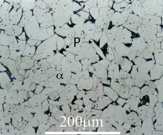 Figure 8: The allotriomorphs have in this slowly cooled low-carbon steel have consumed most of the austenite before the remainder transforms into a small amount of pearlite. Micrograph courtesy of the DoItPoms project. The shape of the ferrite is now determined by the impingement of particles which grow from different nucleation sites
Pearlite is in fact a mixture of two phases, ferrite and cementite (Fe3C). It forms by the cooperative growth of both of these phases at a single front with the parent austenite. In Fe-C systems, the average chemical composition of the pearlite is identical to that of the austenite; the latter can therefore completely transform into pearlite.
In a hypoeutectoid steel, a colony of pearlite evolves with the nucleation of ferrite as illustrated in Fig. 10. This in turn triggers the nucleation of a particle of cementite and this process repeats periodically. The two phases then are able to establish cooperative growth at the common front with the austenite, with much of the solute diffusion happening parallel to this front within the austenite. The distance between the "layers" of cementite and ferrite is known as the interlamellar spacing.
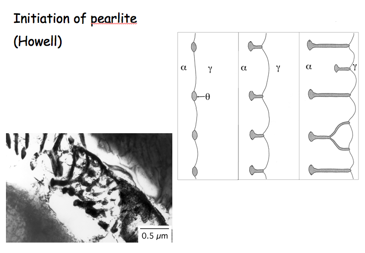 Figure 10: The process by which a colony of pearlite evolves in a hypoeutectoid steel.
The final optical microstructure appears as in Fig. 11, consisting of colonies of pearlite, i.e., regions which participated in cooperative growth at a common front. In this two-dimensional section, each colony appears as if it is a stack of layers of cementite and ferrite. The colonies appear to have different interlamellar spacing, but this may be a sectioning effect.

Indeed, a colony in three dimensions does not consist of alternating, isolated layers of cementite and ferrite. All of the cementite is a single-crystal, as is all of the ferrite. The colony is therefore an interpenetrating bi-crystal of ferrite and cementite. Imagine in Fig. 12, that the cabbage represents in three dimensions, a single crystal of cementite within an individual colony of pearlite. The leaves of the cabbage are all connected in three dimensions. When the cabbage is immersed in a bucket of water, imagine further that the water is a single crystal of ferrite within the same colony of pearlite. The two will interpenetrate to form the bi-crystal.
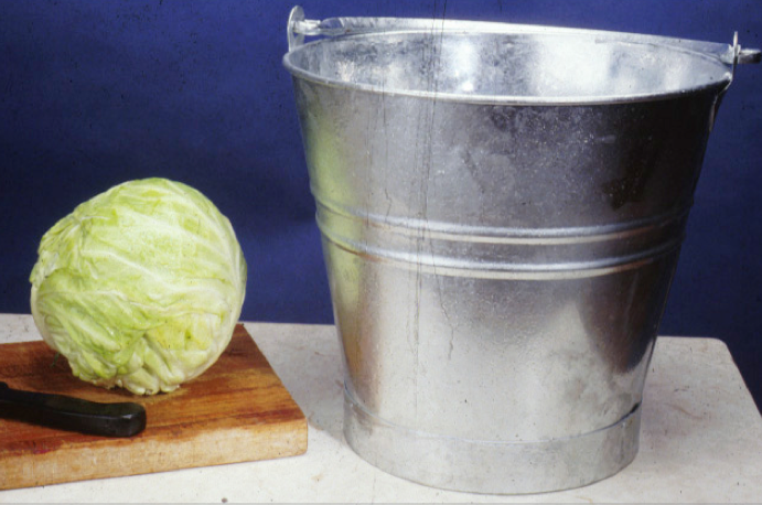 Figure 12: A cabbage and water analogy of the three-dimensional structure of a single colony of pearlite.
It is important to realise that a colony of pearlite is a bi-crystal. Although a steel becomes stronger as the interlamellar spacing is reduced, it does not become tougher because the colony size is what represents the crystallographic grain size. Thus, a propagating cleavage crack can pass undeviated across a colony of pearlite.
Figures 13 and 14 show an optical micrograph and a crystallographic orientation image from the same sample. It is evident from the colour image that the colour (crystallographic orientation) is essentially homogeneous within a colony of pearlite.
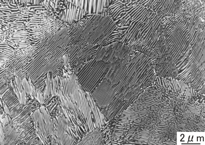 Figure 13: Another optical micrograph showing colonies of pearlite (courtesy S. S. Babu).
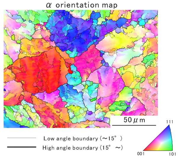 Figure 14: An orientation image of colonies of pearlite (courtesy of S. S. Babu).
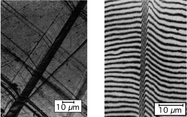
The interlamellar spacing within pearlite can be made fine by growing the pearlite at large thermodynamic driving forces. Figure 15 shows a transmission electron micrograph of pearlite where the interlamellar spacing is about 50 nm. This is well below the resolution of an optical microscope (typically 500 nm). It follows that the lamellae in this case cannot be resolved using optical microscopy, as illustrated in Fig. 16.
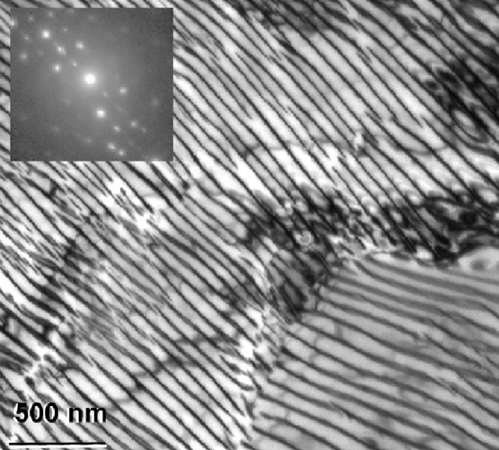 Figure 15: Transmission electron micrograph of extremely fine pearlite.
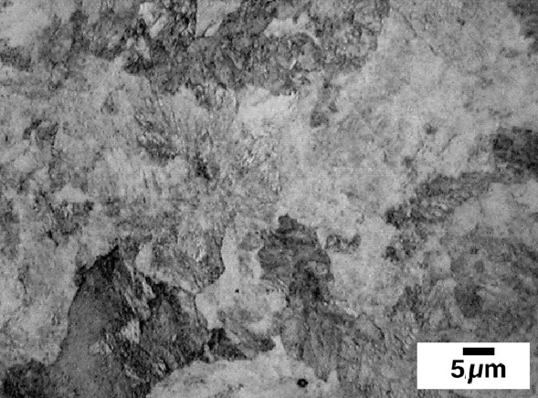 Figure 16: Optical micrograph of extremely fine pearlite from the same sample as used to create Fig. 15. The individual lamellae cannot now be resolved.
Pearlite is a reconstructive transformation which always involves the diffusion of all elements including iron. It cannot happen in the absense of substantial atomic mobility. In alloy steels, in addition to interstitial carbon, the substitutional solutes will partition between the cementite and ferrite. Figure 17 shows this to be the case, with C, Mn and Cr enriching inside the cementite whereas Al and Si partition into the ferrite.
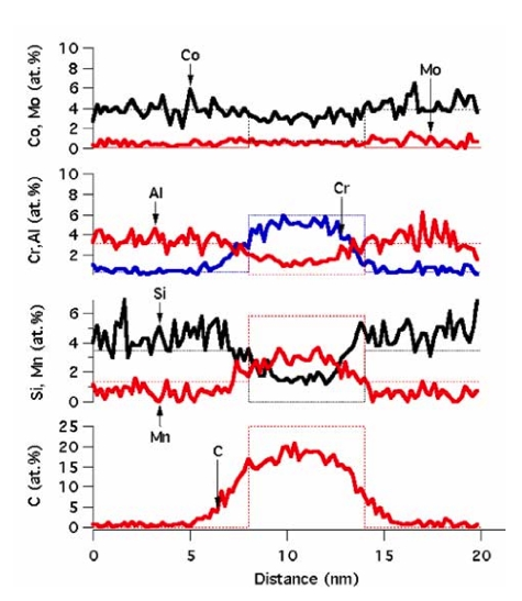 Figure 17: Atom-by-atom chemical analysis across cementite in a pearlite colony. C, Mn and Cr enrich inside the cementite whereas Al and Si partition into the ferrite.
It is sometimes the case that a pearlitic steel is too strong for the purposes of machining or other processing. It can then be heat-treated at a temperature below that at which austenite forms, to allow the cementite to spheroidise. The "lamellae" of cementite turn into approximately spherical particles of cementite in an effort to minimise the amount of θ/α interfacial area/energy per unit volume (Fig. 18).
Since spheroidisation is driven by interfacial area, fine pearlite spheroidises more readily than coarse pearlite. Plastically deformed pearlite which is fragmented will also spheroidise relatively rapidly (Fig. 19).
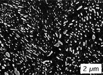 Figure 18: The appearance of an originally pearlitic sample after a spheroidisation heat treatment at 750°C for 1.5 h (courtesy Ferrer et al., 2005).
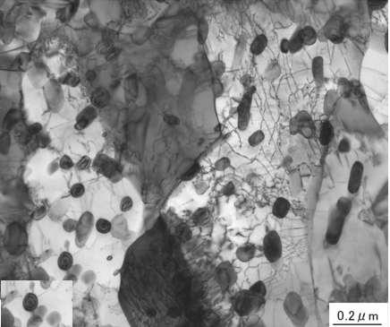 Figure 19: Transmission electron micrograph showing the advanced stages of spheroidisation when plastically deformed pearlite is heat treated at 750°C for 1.5 h (courtesy Ferrer et al., 2005).
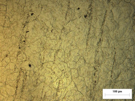
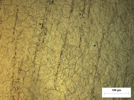
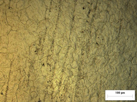
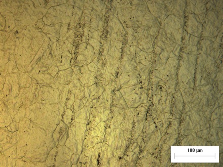
The vast majority of commercial steels contain manganese and are produced by casting under conditions which do not correspond to equilibrium. There are as a result, manganese-enriched regions between the dendrites. Any solid-state processing which involves rolling-deformation is then expected to smear these enriched regions along the rolling direction, thus building into the steel bands of Mn-enriched and Mn-depleted regions.
When the austenite in such steels is cooled, ferrite first forms in the Mn-depleted regions. Ferrite has a very low solubility for carbon which partitions into the Mn-enriched regions which on further cooling, transform into bands of pearlite. The banded microstructure is illustrated in Fig. 20. Fig. 21 shows microanalysis data which confirm that pearlite tends to form in the Mn-enriched regions.
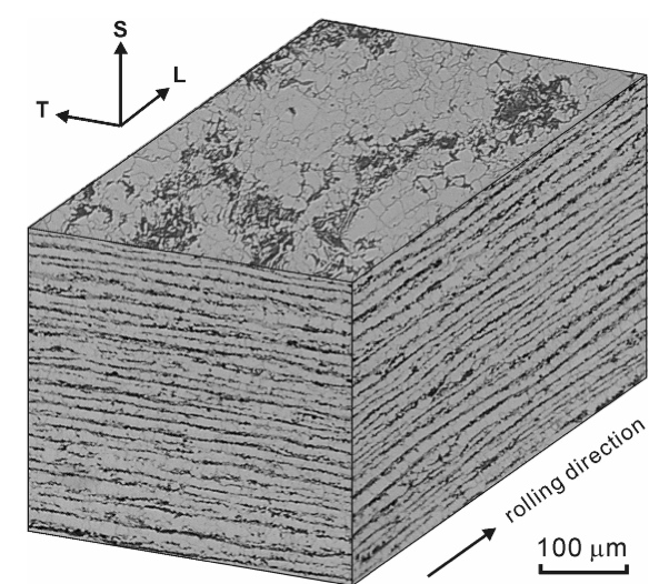 Figure 20: Banded microstructure (courtesy of Professor Yohiharu Mutoh, Nagaoka University of Technology, Japan) "T", "L" and "S" stand for transverse, longitudinal and short-transverse directions respectively. Micrograph courtesy of Y. Mutoh.
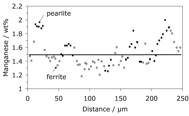 Figure 21: Showing that the manganese depleted regions correspond to ferrite whereas those which are enriched transform into pearlite (courtesy of Howell).
Pearlitic steel can be heat-treated to allow the cementite to spheroidise, minimising the θ/α interfacial energy (Figs. 18, 19). Furthermore, manganese-enriched regions in commercial steels can lead to banded microstructures (Figs. 20, 21).
Martensite transformation begins when austenite is cooled to a temperature below MS on the time-temperature-transformation diagram. It is a diffusionless transformation achieved by the deformation of the parent lattice into that of the product.
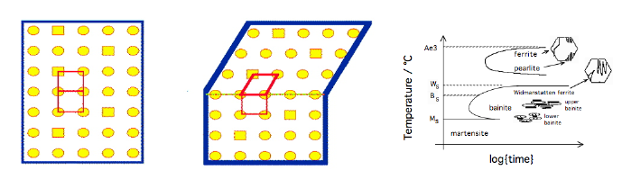
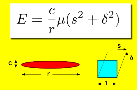
Fig. 23 shows an interference micrograph of a sample of austenite which was polished flat and then allowed to transform into martensite. The different colours indicate the displacements caused when martensite forms. This physical deformation is described on a macroscopic scale as an invariant-plane strain (Fig. 24) consisting of a shear strain s of about 0.25 and a dilatation δ normal to the habit plane of about 0.03.
The strain energy per unit volume, E scales with the shear modulus of the austenite μ the strains and the thickness to length ratio c/r as illustrated in Fig. 24. The martensite therefore forms as a thin plate in order to minimise the strain energy. All of the displacive transformation products are therefore in the form of thin plates.
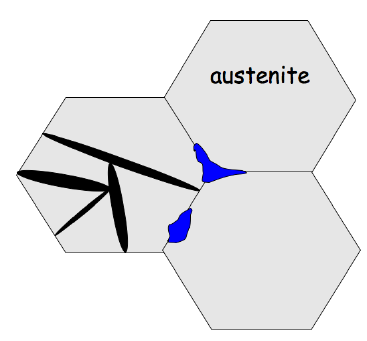
We have emphasised that the discipline motion of atoms cannot be sustained across austenite grain boundaries and hence plates of martensite, unlike allotriomorphs, are confined to the grains in which they nucleate (Fig. 25).
The austenite grain boundaries are thus destroyed in the process of forming allotriomorphic ferrite or pearlite. This is not the case with displacive transformation products where even if all the austenite is consumed, a vestige of the boundary is left as the prior austenite grain boundary. Austenite grain boundaries and indeed, prior austenite grain boundaries, absorb detrimental impurities. One consequence is that strong steels based on microstructures obtained by displacive transformation become susceptible to impurity embrittlement.
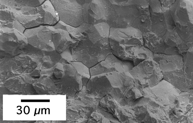
Fig. 26 shows the form of the fracture surface expected when failure occurs due to impurity embrittlement at the prior austenite grain boundaries. The grains simply separate at the grain surfaces with little absorption of energy during fracture.
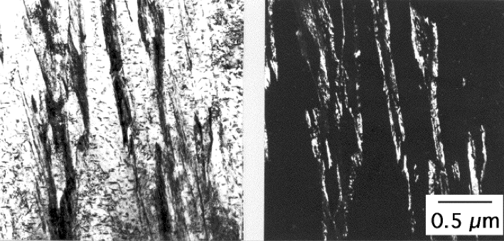
In alloys containing large concentrations of solutes (for example, Fe-1C wt% or Fe-30Ni wt%), the plate shape of martensite is clearly revealed because substantial amounts of retained austenite are present in the microstructure, as illustrated in Fig. 27. In contrast, lower alloy steels transform almost completely to martensite when cooled sufficiently rapidly. Therefore, the microstructure appears different (Fig. 28) but still consists of plates or laths of martensite.
Transmission electron microscopy can reveal the small amount of inter-plate retained austenite in low-alloy steels (Fig. 29).
Tempering at a low temperature relieves the excess carbon trapped in the martensite, by the precipitation of cementite. The retained austenite is not affected by tempering at temperatures below MS, Fig. 30.
In some steels containing a strong carbide-forming elements such as Mo or V, tempering at temperatures where these solutes are mobile leads to the precipitation of alloy carbides (Fig. 31).
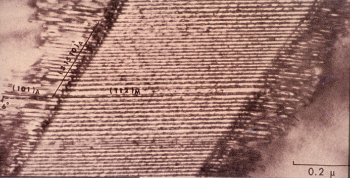
The Bain strain which converts austenite into martensite is a huge deformation; to mitigate its effects there are other deformations which accompany the transformation. These change the overall shape deformation into an invariant-plane strain. One consequence is that there are lattice invariant deformations such as slip and twinning on a fine scale. Slip simply leads to steps in the interface, whereas twinning also introduces interfaces inside the martensite plate, as illustrated in Fig. 32.
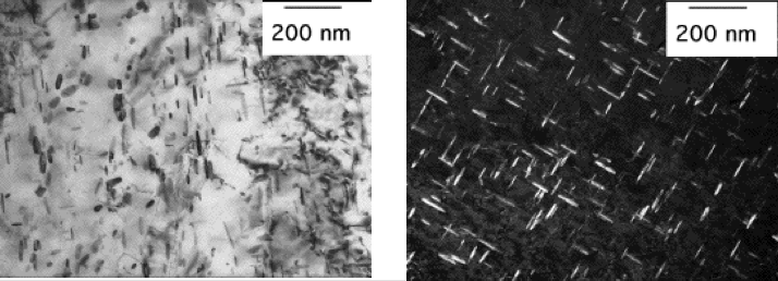
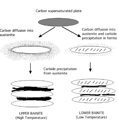
The atomic mechanism of bainite is similar to that of martensite (Fig. 33). Plates of bainite form without any diffusion, but shortly after transformation, the carbon partitions into the residual austenite and precipitates as cementite between the ferrite platelets - this is the structure of upper bainite (Fig. 34). Lower bainite is obtained by transformation at a lower temperature; the carbon partitioning is then slower, so some of the excess carbon has an opportunity to precipitate inside the ferrite plates and the rest of it precipitates from the carbon-enriched austenite as in upper bainite, Fig. 34.
The difference between bainite and martensite is at primarily at the nucleation stage. Martensitic nucleation is diffusionless, but it is thermodynamically necessary for carbon to partition during the nucleation of bainite. Bainite also forms at temperatures where the austenite is mechanically weak. The shape deformation due to the bainite transformation is therefore casues plastic deformation in the adjacent austenite. This deformation stops the bainite plates from growing and transformation then proceeds by the nucleation of further plates, which also grow to a limited size.
We have categorised transformations into displacive and reconstructive, with the former being strain dominated and the latter diffusion dominated. Displacive transformations are also known as military transformations by analogy to a queue of solidiers boarding a bus. The soliders board the bus in a disciplined manner such that there is a defined correspondence between their positions in the bus and those in the queue. Near neighbours remain so on boarding. There is thus no diffusional mixing and no composition change. Because the soldiers are forced to sit in particular positions, there will be a lot of strain energy and this is not an equilibrium scenario.
A civilian transformation is one in which the queue of civilians board the bus in an un-coordinated manner so that all correspondence between the positions in the bus and the queue is lost. Civilians occupy the positions they prefer to occupy, a situation analogous to diffusion.
There is a third kind of transformation, paraequilibrium in which the larger atoms in substitutional sites move in a discipline manner (without diffusion) whereas the faster moving interstitial atoms diffuse and partition between the phases. This is how Widmanstätten ferrite grows, a displacive mechanism whose rate is controlled by the diffusion of carbon in the austenite ahead of the αw/γ interface.
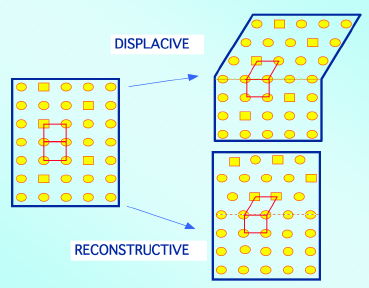
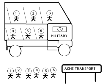
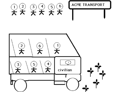
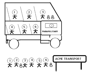
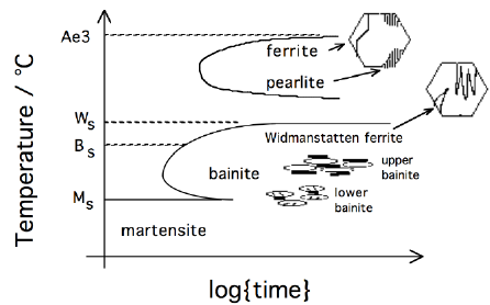 Figure 37: Widmanstätten ferrite on the time-temperature-transformation diagram.
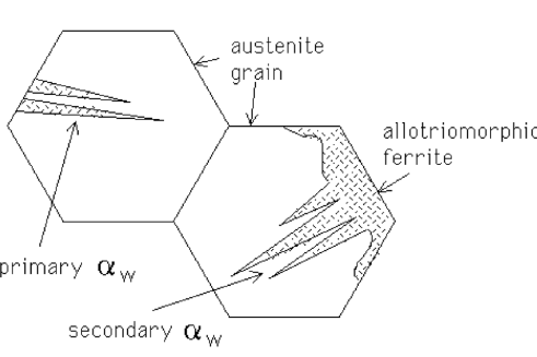 Figure 37: Widmanstätten ferrite on the time-temperature-transformation diagram.
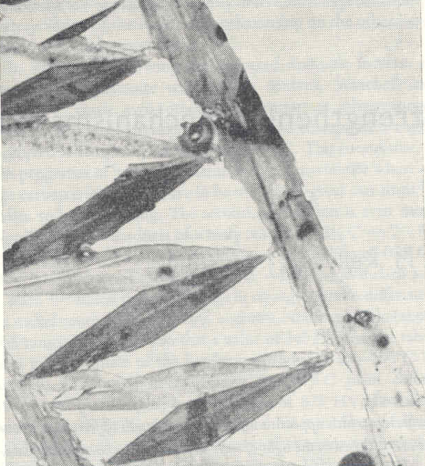
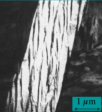
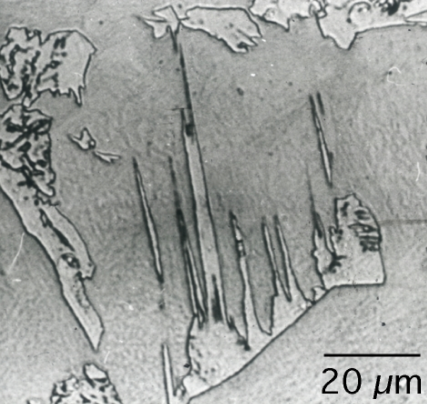 Figure 39: Optical micrographs showing white-etching (nital) wedge-shaped Widmanstätten ferrite plates in a matrix quenched to martensite. The plates are coarse (notice the sacle) and etch cleanly because they contain very little substructure.
In fact, the strain energy due to the shape deformation when an individual plate of Widmanstätten ferrite forms is generally so high that it cannot be tolerated at the low driving-force where it grows. As a consequence, two back-to-back plates which accommodated each others shape deformation grow simultaneously. This dramatically reduces the strain energy, but requires the simultaneous nucleation of appropriate crystallographic variants. As a consequence, the probablity of nucleation is reduces and the microstructure is coarse. The characteristic thin-wedge shape of αw is because the two component plates have different habit plane variants with the parent austenite.
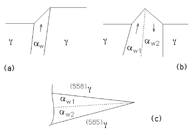
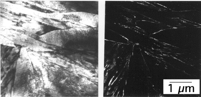
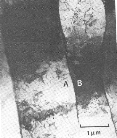 Figure 42: Transmission electron micrograph of what optically appears to be single plate, but is in fact two mutually accommodating plates with a low-angle grain boundary separating them.
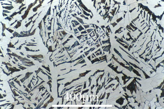
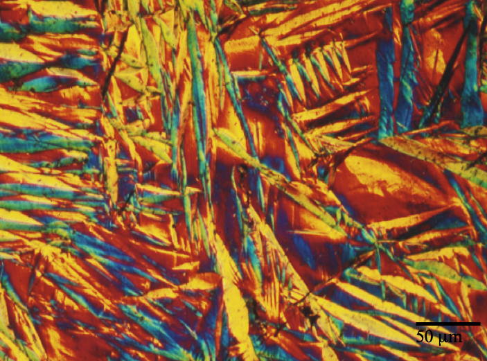
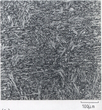
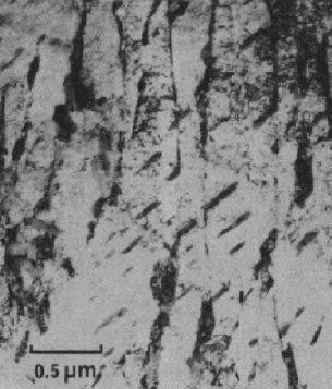
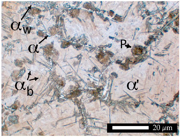
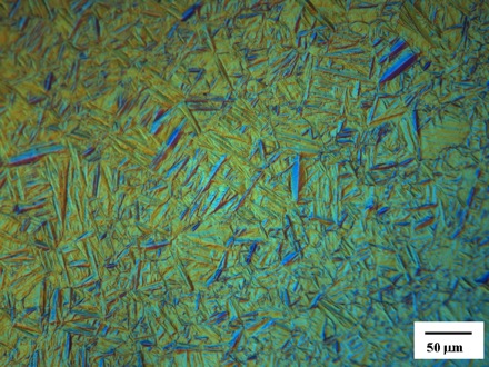
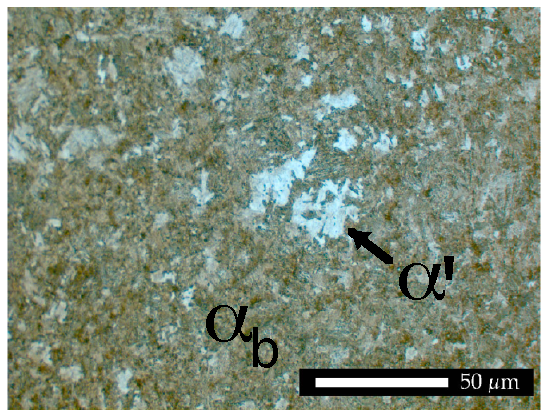 Figure 44: Optical micrograph of a mixed microstructure of bainite and martensite in a medium carbon steel. The bainite etched dark because it is a mixture of ferrite and cementite, and the αb/θ interfaces are easily attacked by the nital etchant used. The residual phase is untempered martensite which etches lighter because of the absence of carbide precipitates.
 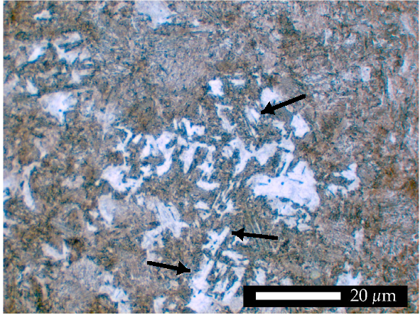 Figure 45: Notice the straight edges (arrowed) to the light-etching areas of martensite. These are also characteristic of a mixed microstructure of bainite and martensite, because bainite forms on specific crystallographic planes of austenite. The edges would not be so straight if the brown-etching phase was pearlite.
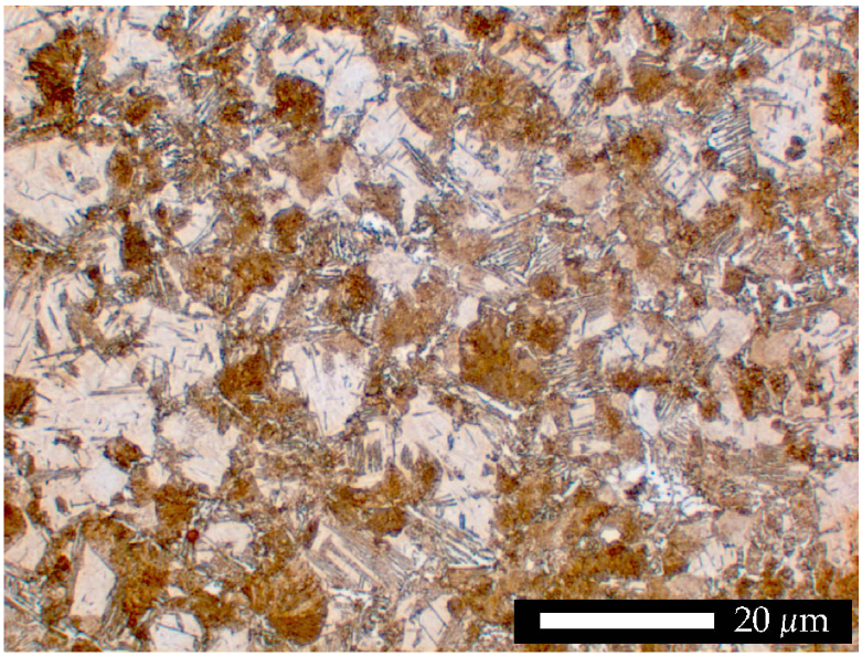
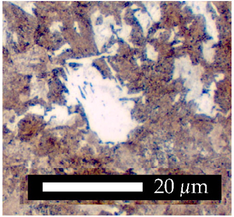 Figure 46: A higher magnification optical micrograph of a mixture of bainite and martensite. The straight edges are clear, and it is even possible to see the occasional bainite plate inside the light-etching phase which was originally austenite but is now untempered martensite.
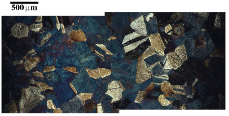
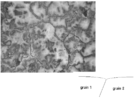
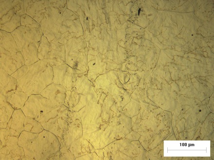
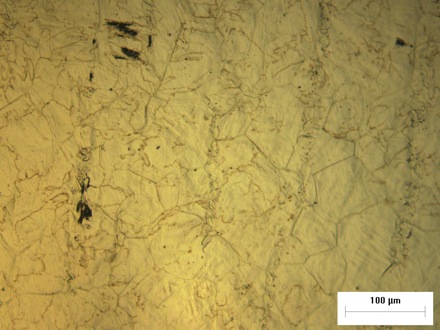
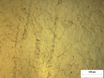
The following micrographs are courtesy of Arijit Saha Podder. The samples were polished to a mirror finish prior to heat treatment. The thermal grooves reveal the austenite grain boundary structure. The photographs are taken using ordinary reflected light microscopy. Here the sample is transformed to allotriomorphic ferrite to avoid surface relief effects.
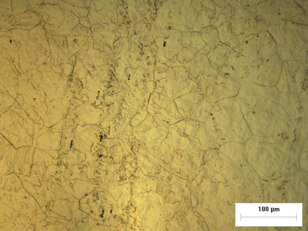
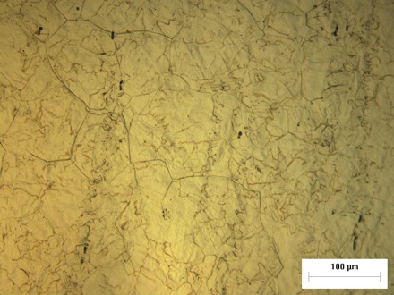
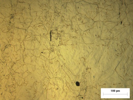
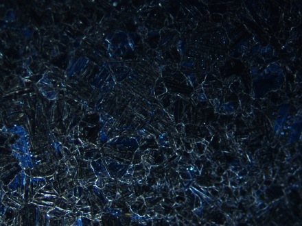
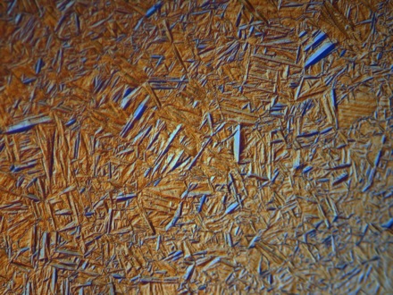
The following micrographs are courtesy of Arijit Saha Podder. The samples were polished to a mirror finish prior to heat treatment. The thermal grooves reveal the austenite grain boundary structure. The photographs are taken using Nomarsk interference light microscopy. Here the sample is transformed into martensite, so the surface relief effects complicate visualisation of the prior austenite grain boundaries.
Images taken by Laura Pocock, of a martensitic weld metal with an extremely fine structure, with individual plates of martensite being about 0.2 micrometres in thickness. These kinds of structures are difficult to index during electron backscattered diffraction. For example, the electron beam spreads within the sample, thereby compromising crystallographic resolution.
The problem can be solved by using transmission electron microscopy to conduct the crystallographic analysis, however, this limits the size of the region than can be examined.
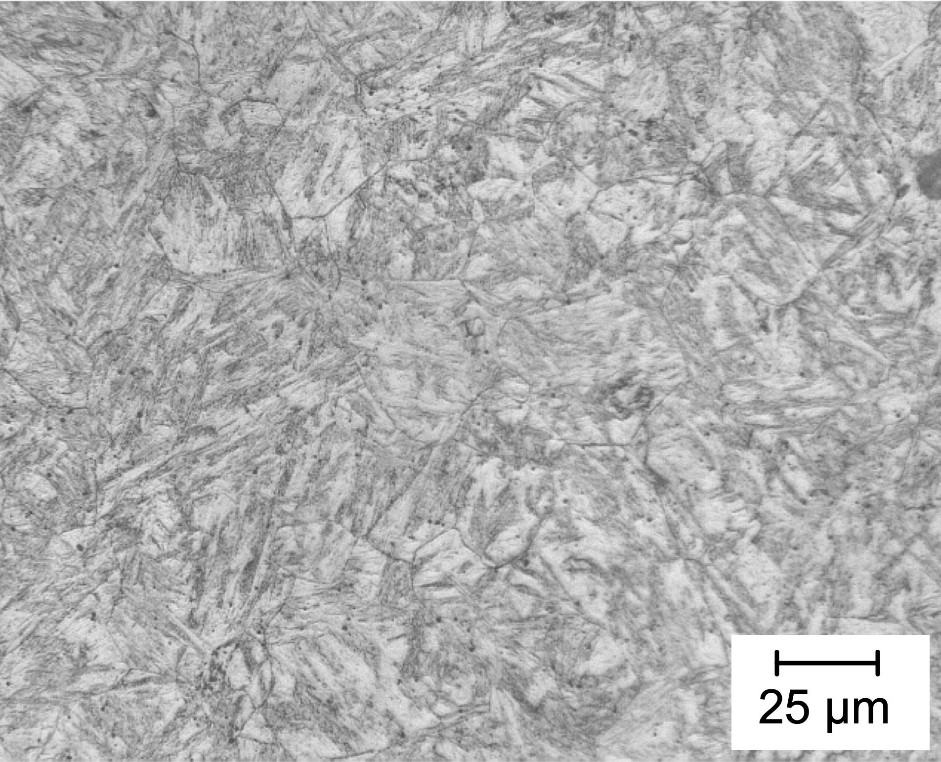
Optical micrograph of a martensitic weld metal. Chemical composition Fe-0.014C-12.7Cr-5.3Ni-1.4Mn-0.1Mo wt%.
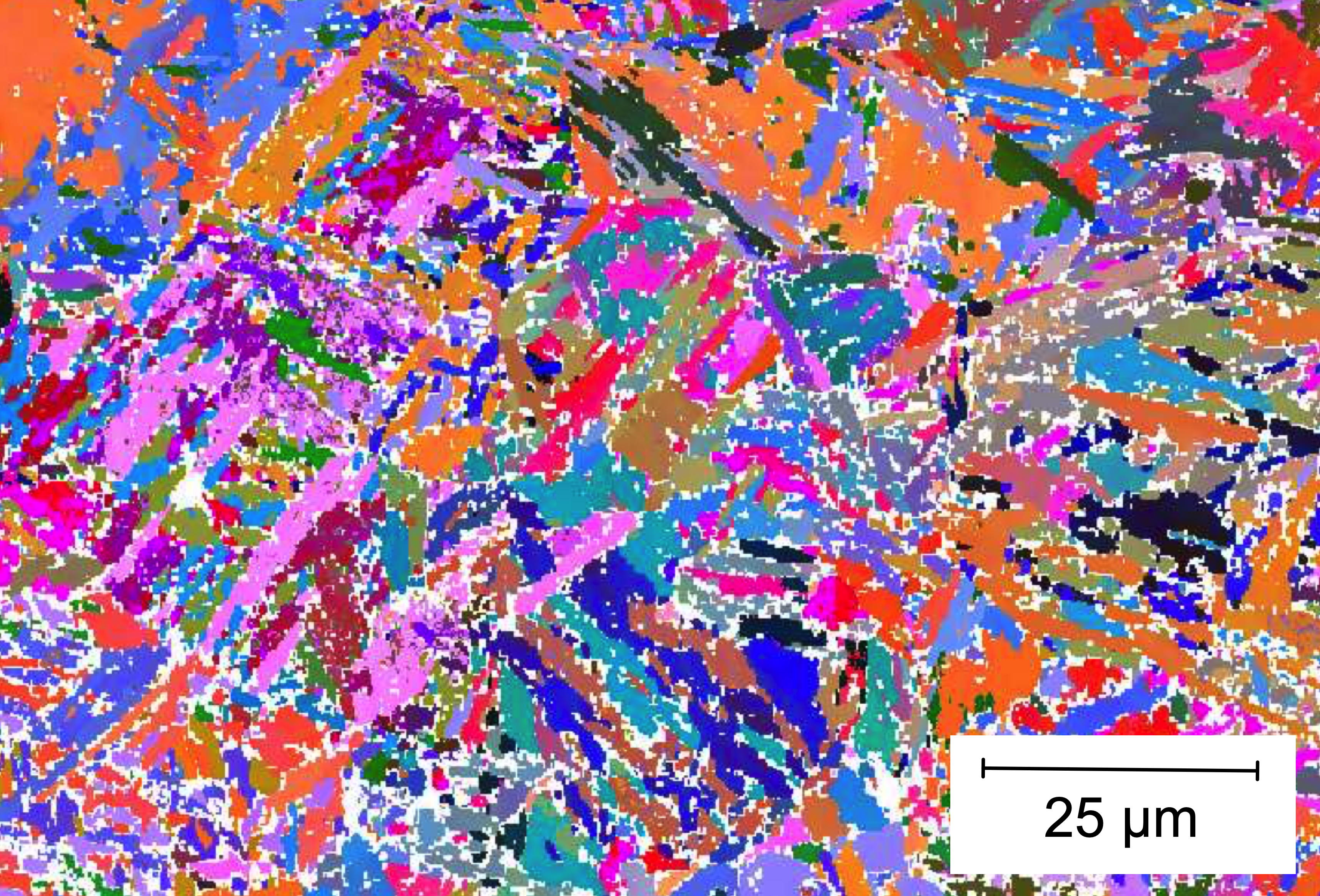
Euler map illustrating crystallographic orientations, on the same sample, mechanically ground and polished sample and then electropolished using a 92% acetic acid and 8% perchloric acid solution at 40 V. About a quarter of the image is not indexed using a step size of 0.2 micrometres. Bear in mind that an individual plate of martensite will be on that scale, so the regions that are uniformly coloured represent clusters of plates in similar orientations, not individual plates.