Biogenesis - introduction
Once a neural network model has been created, it is frequently desirable to use the model backwards and identify sets of input variables which result in a desired output value. The large numbers of variables and non-linear nature of many materials models can make finding an optimal set of input variables difficult.
Here, we can use a genetic algorithm to try and solve the problem.
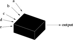
What are genetic algorithms? Genetic algorithms (GAs) are search algorithms based on the mechanics of natural selection and genetics as observed in the biological world. They use both direction (“survival of the fittest”) and randomisation to robustly explore a function. Importantly, to implement a genetic algorithm it is not even necessary to know the form of the function; just its output for a given set of inputs (Figure 1).
What do we mean by robustness? Robustness is the balance between efficiency and efficacy necessary for a technique to be of use in many different environments. To help explain this, we can compare other search and optimisation techniques, such as calculus-based, enumerative, and random searches.
Calculus-based approaches assume a smooth, unconstrained function and either find the points where the derivative is zero (easier said than done) or follow a direction related to the local gradient to find the local high point (hill climbing). These techniques have been heavily studied, extended and rehashed, but it is simple to demonstrate their lack of robustness.
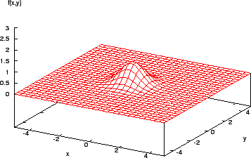
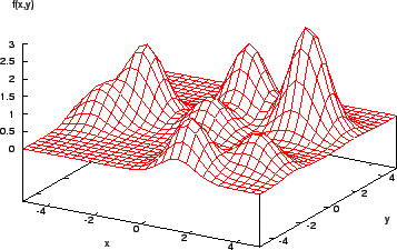
Consider the function shown in Figure 2. It is easy for a calculus-based method to find the maximum here (assuming the derivative of the function can be found!). However, a more complex function (Figure 3) shows that the method is local - if the search algorithm starts in the region of a lower peak, it will miss the target, the highest peak.
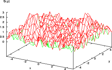
Once a local maximum is reached, further improvement requires a random restart or something similar. Also, the assumption that a function is smooth, differentiable, and explicitly known is seldom respected in reality. Many real-world models are fraught with discontinuities and set in noisy multimodal search spaces (Figure 4).
While calculus-based methods can be very efficient in certain environments, the inherent assumptions and local nature means they are insufficiently robust across a wide spectrum of problems.
In such cases, it may be tempting to try and calculate the whole surface and find maxima that way. This brute force method is, unsurprisingly, highly inefficient. Alternatively, a random-walk approach may be used to explore the surface. This is also inefficient - although both of these methods retain their applicability across a wide range of problem types, unlike the calculus-based approach.
How, then, do genetic algorithms (GAs) differ from these methods? Drawing from biological genetics and natural selection, there are three fundamental differences:
- GAs search from a population of points, rather than a single point.
- GAs use an objective function only, rather than derivatives or other additional information about the search space.
- GAs use probabilistic rules rather than deterministic rules.
This combination of properties allows a large, multi-parameter space to be explored efficiently and efficaciously, provided they are applied judiciously.
Evolution - using genetic algorithms
To start with, it is necessary to encode the parameter set for a model into a chromosome, $X_i$. This is a way of expressing the information that allows for various forms of mutation to occur in the parameter set, and consists of a set of genes, $[x_{i1}, x_{i2}, x_{i3}, x_{i4}, \dots]$. This set of genes, when given to the model as inputs, will give the output $f_i$. The chromosomes are then ranked according to a fitness factor, $F_i$, describing how well they perform relative to expectation and each other.
The chromosomes are then allowed to breed (with a likelihood proportional to fitness) and mutate. In practice, evolution occurs in two ways - crossover (see Tables 1 and 2) and random variation. In this example, mutation would be represented by flipping a randomly chosen bit. In a neural network optimisation GA, mutation would involve a small variation - plus or minus - in a randomly chosen gene.
| String no. | String | $F_i$ | $\frac{F_{i}}{\Sigma{}F_{i}}$ | No. surviving | Mating pool |
|---|---|---|---|---|---|
| 1 | 01101 | 169 | 0.14 | 1 | 01101 |
| 2 | 11000 | 576 | 0.49 | 2 | 11000 |
| 3 | 01000 | 64 | 0.06 | 0 | 11000 |
| 4 | 10011 | 361 | 0.31 | 1 | 10011 |
| Mating pool | Mate | Crossover site | New population | New $F_i$ |
|---|---|---|---|---|
| 0110−1 | 2 | 4 | 01100 | 144 |
| 1100−0 | 1 | 4 | 11001 | 625 |
| 11−000 | 4 | 2 | 11011 | 729 |
| 10−011 | 3 | 2 | 10000 | 256 |
This simple example demonstrates a basic optimisation problem. For complex multi-parameter models, larger populations will be necessary for efficient exploration of the parameter space and, to further increase efficiency, multiple populations may be used. This allows a range of forms of variation to occur with every generation. Typically, say, from a population of 20 chromosomes, for the next generation the best (fittest) may be preserved unchanged (elitism); a further 18 places, for crossover and mutation, may be randomly filled based on their relative fitnesses (as in Table 1); and the final place filled by a completely new, randomly generated chromosome.
To summarise, the process is:
- Select an initial population.
- Rank population according to fitness.
- Randomly select mating pairs from population according to fitness.
- Breed from mates with crossover1 and mutation.
- If desired, fill remaining gaps in new generation with the best performer of the previous generation and/or newly generated members.
- Goto (2).
The algorithm is repeated until:
- a solution is found that satisfies a target
- a fixed number of generations has been produced
- the highest ranking solutions reach a plateau and there is no further improvement with repeated iteration, or
- you run out of time and/or money.
Speciation - genetic algorithms for Bayesian neural networks
For Bayesian artificial neural networks (ANNs), we have a set of input parameters and two output values - the prediction from the network and its associated uncertainty. Assuming that we want to avoid wild predictions, we can use a fitness function $F_i$ which incorporates both of these outputs, for example:
where:
in which $L$ is the number of models in the predicting committee, $\sigma_{y}^{(l)}$ is the uncertainty associated with the prediction of each committee member $l$, $t$ is the target output for the optimisation, and $f_i$ is the committee prediction.
The basic chromosome, as mentioned above, can consist of the set of inputs to the network.
There are some ways to help optimise the procedure when applied to ANNs. The first is that it is desirable to avoid finding an “optimal” input set with non-physical values. As all inputs are normalised before the neural network is applied, it is perfectly possible to make predictions for a steel containing -1 wt% carbon, for example. This can be avoided in two ways - by restricting the range of the genes during “mutation” and the generation of new chromosomes, or by adding terms to the fitness function to additionally penalise such unphysical genes and hence use evolution against them.
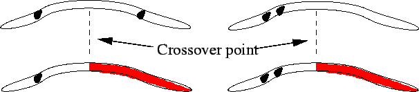
In addition, because single-point crossover efficiently selects for combinations of genes that are close together in the chromosome but tends to split up combinations that are far apart (Figure 5), inputs that are likely to have a combined effect should be grouped close to one another in the chromosome. This effect can be avoided by using uniform crossover - selecting genes at random from either parent (Figure 6) - although this will make the algorithm less efficient at finding very “fit” combinations.
| Parents | Crossover mask | Offspring |
|---|---|---|
| 12345 | 11221 | 12895 |
| 67890 |
It is also common to have, as inputs to an ANN model, variables which are functions of other input variables, such as, say, Arrhenius forms like $\exp\left(\frac{-1}{kT}\right)$ as well as the temperature itself. In this case care must be taken that one is always a function of the other, and that they are not allowed to vary independently. We may additionally have a number of input variables which we wish to keep constant - if we are trying to optimise a steel for performance at a particular temperature, say.
Colonisation - optimising the algorithm
In a simple genetic algorithm run, there are a number of basic parameters, as shown in Table 3.
| Computing parameters | GA parameters |
|---|---|
| Number of populations | Crossover rate |
| Number of generations | Mutation rate |
| Rate of population mixing | |
| Population size |
Table 3: The basic parameter set for a genetic algorithm optimisation.
The computing parameters are simple - using additional populations allows multiple areas of the network to be explored at once but increases the computing power required - and how long do you need to run the procedure for? The GA-specific parameters require a little more explanation, although population size is self-explanatory.
The crossover rate is the proportion of each new generation which undergoes crossover. The mutation rate is the rate at which mutations occur. In optimising a neural network model, we need a relatively high mutation rate, where a mutation is a small nudge $\delta\sigma$ of a gene value. The rate of population mixing is the frequency that different populations are allowed to undergo crossover.
The effects of these parameters are explored in Delorme (2003)2. To summarise, 3 populations of 20 chromosomes running for 3000 generations is a good start for many Bayesian neural network optimisations, with a crossover rate of 90% (i.e. for a population of 20, 18 chromosomes are chosen using the roulette wheel method and crossed with another 18 using the same method, producing 18 offspring). The remaining slots are filled with the best performer from the previous population, and a wholly new randomly-generated chromosome. Every generation, one gene in the population is mutated.
The preservation of the elite performer simulates some of the features of local-maximum search techniques, allowing the optimal chromosome found so far to be preserved in the population unchanged. This can occasionally lead to the algorithm getting “stuck” at a sub-optimal solution if the model is very multi-modal, but the use of multiple populations and a high mutation rate minimise this probability, as does the inclusion of a new set of genes in every generation.
The Tarpits - potential pitfalls
The chief problems associated with GA optimisation are:
- Application to constrained problems.
- GA deceptive functions.
- Premature convergence.
- Lack of convergence towards the end of an optimisation.
- An overly high mutation rate.
- The meaning of fitness.
A constrained problem is one in which there are limits to the values that can be used as inputs to the network (such as a chemical composition which cannot be negative), although the nature of ANNs and GAs are naturally unconstrained. Two ways to fix this problem are mentioned above - restriction of the mutation process or modification of the fitness function to reflect the constraints and penalise those chromosomes that transgress them.
GA deceptive functions are functions which confound the GA by selecting for an individual gene at the expense of another gene, when a combination of the two would lead to optimal fitness. This leads, in some cases, to the elimination from the genepool of optimal values of those genes. This can be avoided by elitism (as mentioned above), the use of multiple populations, and a high mutation rate to reintroduce any genes lost.
Premature convergence is a similar problem - if a chromosome is far fitter than its rivals early on, it can come to dominate a population, leading to loss of genes which may, later, lead to better solutions. This can be avoided by employing a high mutation rate, and also through fitness scaling. This is a process that re-scales the absolute $F_i$ with respect to the average of the population, so that the fittest chromosome is only, say, twice as likely to be chosen for cross-breeding as the average chromosome.
This procedure also aids the problem of lack of convergence towards the end of an optimisation procedure. In this case, a population of similarly high-performing chromosomes will not compete strongly with one another. Fitness scaling here retains the competition between chromosomes and keeps the algorithm efficient. A potential danger is that any poor performers left in the population may end up with negative $F_i$ after re-scaling. In this case, these chromosomes can be assigned a fitness of zero.
An overly high mutation rate makes the process inefficient, as the GA then starts to resemble a random walk rather than a directed process.
Lastly, some thought must be given to the meaning of “fitness”. When designing a genetic algorithm, what do you actually want it to do? For finding a set of optimal values that will give a specific output from a neural network, the answer is easy. When applying GAs to other problems, defining an appropriate fitness function can make all the difference between success and an unexpectedly random result.
Example
A neural network model was created to predict the effect of irradiation on the yield stress (YS) on a class of steels known as reduced-activation ferritic/martensitic (RAFM) steels3. In order to find alloys which exhibited moderate irradiation hardening, a genetic algorithm was used.
Inputs to the neural network included chemical composition, irradiation temperature and damage level, tensile test temperature, radiation-induced helium levels, and degree of cold working prior to irradiation. In this case, all we were interested in was an optimised ideal chemical composition. Therefore, all other parameters were fixed (including compositional impurity levels). In addition, the Cr content was fixed - Cr strongly affects radiation embrittlement with a minimum around 9 wt% Cr, and this was a rough attempt to optimise for both properties without having to extensively modify existing GA code.
The chromosome therefore consisted of the major alloying elements in RAFM steels: C, W, Mo, Ta, V, Si and Mn. 3 populations of 20 chromosomes were randomly generated from within appropriate limits for each gene. The program then went through following loop for each population:
- Convert the chromosomes to a set of neural network inputs by combining them with the fixed inputs (irradiation temperature etc.).
- Make predictions on each set of inputs, and convert the predictions and uncertainties to fitnesses, using Equation 1.
- Rank the chromosomes by fitness.
- Preserve the best chromosome (elitism).
- Create 18 new chromosomes by crossbreeding using the roulette wheel algorithm. For this calculation, uniform crossover was used.
- Create one new chromosome at random (within appropriate limits for each gene).
- Mutate one randomly chosen gene in the entire population by adding or subtracting a small amount (1% of the training database range for that input). If the mutation makes the gene non-physical (less than zero in this case), set it to a default physical value (zero in this case).
- Return to (1) with the new population.
Every 400 generations, the best performer in each population was allowed to crossbreed with the best performers from each other population. This was to prevent any populations getting stuck in a local (rather than a global) maximum. The calculation was run for 3000 generations in total, which took about 2-and-a-half weeks. The results for a 20 dpa4 irradiation at 700 K are shown in Table 4.
| Input | Eurofer97 | Best results from population | ||
|---|---|---|---|---|
| Reference alloy | 1 | 2 | 3 | |
| C | 0.1 | 0.144 | 0.144 | 0.144 |
| Cr | 9.0 | 9.0 | 9.0 | 9.0 |
| W | 1.1 | 1.78 | 1.78 | 1.78 |
| Mo | 0.0 | 0.50 | 0.50 | 0.50 |
| Ta | 0.15 | 0.27 | 0.27 | 0.27 |
| V | 0.2 | 0.15 | 0.15 | 0.15 |
| Si | 0.0 | 0.185 | 0.185 | 0.185 |
| Mn | 0.0 | 0.0 | 0.0 | 0.0 |
| Target YS /MPa | 450 | 600 | 600 | 600 |
| Prediction /MPa | (unirradiated) | 607 | 607 | 607 |
| Uncertainty /MPa | - | 198 | 198 | 198 |
The fact that all three populations predict very similar results (there were some differences in the third decimal places) strongly suggests that this is a global maximum fitness. Note, though, that this is not necessarily the lowest possible yield stress in the ANN model, but the closest to the target YS, given the additional constraints (i.e. the fixed inputs not in the chromosome).
It is of course possible to create a fitness function which takes into account multiple properties from multiple network models and optimises for all of them, although this has not yet been done in our group.
Sample questions
There are some simple questions to test understanding of the basic concepts here.
Recommended reading
Genetic Algorithms in Search, Optimization and Machine Learning by David Goldberg (pub. Addison Wesley, 1989) is an excellent overview of the field and the theory behind it.
A GA code for neural networks is also available through the MAP website:
https://www.phase-trans.msm.cam.ac.uk/map/mapmain.html
Bibliography
- Minsung Joo, 2008, Reducing redundancy in steel design, M.Eng. Thesis, POSTECH
- D E Goldberg. Genetic algorithms in search, optimisation, and machine learning. Addison Wesley, 1989.
- Shah, I., 2002, Tensile Properties of Austenitic Stainless Steel, I. Shah, M.Phil. Thesis, University of Cambridge
- Delorme, A., 2003, Genetic Algorithm for Optimization of Mechanical Properties, Technical report, University of Cambridge
- Slide presentation, Richard Kemp
- Slide presentation, Tracey Cool
Computer programs
- Application of the genetic algorithm (GA) for reaching a solution given a fitting function. This can in theory be applied to any problem, where a database of inputs and outputs has trained a neural network.
- This program is an implementation of a genetic algorithm which can reach an optimum set of parameters for a target value of yield strength of austenitic stainless steel. This can in theory be applied to any problem, where a neural network exists.
- This program is an implementation of a genetic algorithm which can reach domains of inputs, such as chemical composition and processing variable, for a desired target value of the elongation to failure of hot-rolled steel. This can in theory be applied to any problem, where a database of inputs and outputs has trained a neural network.
- This program is an implementation of a genetic algorithm which can reach optimum sets of input parameters, such as chemical composition and processing variable, for two desired target values of the ultimate tensile strength and the elongation to failure of hot-rolled steels in the same time. This can in theory be applied to any problem, where a neural network exists.
- This program is an implementation of a genetic algorithm which can reach domains of inputs, such as chemical composition and processing variable, for a desired target value of the ultimate tensile strength of hot-rolled steel. This can in theory be applied to any problem, where a database of inputs and outputs has trained a neural network.
Acknowledgements
The creation of this document was supported by the Higher Education Funding Council for England, via the U.K. Centre for Materials Education.
June 5th 2006
Footnotes
- 1. crossover
- The mutation and crossover operators mentioned here are a very condensed list of all the techniques that have been explored since GAs were first developed in the 1970s.
- 2. delorme2003
- Available via https://www.phase-trans.msm.cam.ac.uk/
- 3. steels
- This model is also available via the MAP website - see Recommended Reading.
- 4. 20 dpa
- “Displacements per atom” - a way of measuring irradiation damage.